Universal Framework for Science and Engineering - Part 2: Regression

• Download code - 1.13 MB
• Download installer - 1.19 MB
• Download documentation - 1.67 MB
• Download installer of Hipparcos and Tycho catalogue of stars - 209 Kb
• Download sample of construction of Herzsprung-Rassel diagram - 6.61 Kb
• Download sample of determination of 6D position of 3D objects by photos - 56.3 Kb
• Download sample of identification of parameters of a control system - 7.17 Kb

Introduction

This article is written based on request from readers for concrete examples of the Universal Framework for Science and Engineering. We shall consider a class of scientific problems related to regression. I'll show how this framework solves problems in astronomy, control systems, and navigation.

Background

The common approaches to the framework have been considered in my previous article. Now, I'll consider application of the framework to regression. Nonlinear regression in statistics is the problem of fitting a model.

to multidimensional x,y data, where f is a nonlinear function of x, with regression parameter θ.

Nonlinear regression operates with selections. This software implements two methods of manipulation with selections. The first method loads selection iteratively, i.e., step by step. The second one loads selection at once.

The architecture of nonlinear regression software that uses iterative regression is presented in the following scheme:

Let us describe the components of this scheme. The iterator provides data-in selections x and y. The y is the Left part of fitting the equations. The Transformation corresponds to the nonlinear function f, and generates the Left part of the fitting model. The Processor coordinates all the actions and corrects the Regression parameters.

The architecture of the software with loading selection at once is presented in the following scheme:

The processor compares Calculated parameters with Selection, calculates residuals, and then corrects Regression parameters. In these two schemas, the Iterator, Selection, and others are not concrete components. They are components that implement interfaces of Iterator, Selection etc. For example, a Camera component may implement the Selection interface. Here, I'll consider examples in brief. A more profound description is available in the documentation of this project.

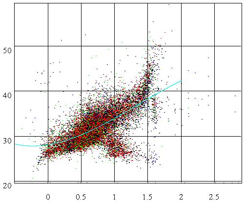
Example 1. Herzsprung-Rassel Diagram

One of the most valuable methods of astronomy is statistics. The statistics enables scientists to find different relations between the parameters of the stars. The discovery of the relation between an absolute star magnitude and its brightness is very valuable in astronomy. This relation is known as the Herzsprung-Rassel diagram. I'll reproduce this discovery using a recent star catalogue Hipparcos and my framework. This research corresponds to the following combination of components of the framework:

Let us shortly describe them. First one is a Data that has the icon. The editor of the properties of this component is presented in the following picture:

It contains the SQL query for the necessary selection. The Filter component performs additional filtration for selection. It contains the logical expression:

This expression means that the parallax exceeds b (b = 200), and the error of parallax is more than three times exceeding the parallax error. The Formula and Regression components enable us to use the necessary formulas. The Processor component is a coordinator of the regression process. Its editor of properties is presented below:

It enables us to set the regression parameters and the regression equations. If you click the Iterate button, then the Processor shall perform an iteration of nonlinear regression. The components Circles and Graph enable us to indicate the Herzsprung-Rassel diagram and its regression curve (see the picture at the beginning of this document). If you wish to try this example, you need to install Tycho and the Hipparcos database and then open this file using the framework.

Example 2. Determination of the 6D Position of a 3D Object by Photos

If we have a several sets of photos of a 3D object, we can obtain its 6D position. In this example, this problem is solved by the following way. From the photos and virtual cameras, we obtain the contours of the object as it is presented in the following picture:

The red contour corresponds to the photo, and the blue one corresponds to the virtual 3D Object. Then, we perform a virtual 6D motion of the object to match both contours. As a result, we have a matching that looks like:

For solving this problem, we will use the following combination of components:

A profound description of this combination is contained in section 8.4 of the product documentation. Here, I'll describe it in brief. The Plane component corresponds to a binary file of the 3D object. I use a special file format for it. Three virtual cameras draw this object using OpenGL graphics (the graphics driver may be easily changed). The editor for the properties of the camera looks like:

The component constructs the contours. We also have the State Frame moved reference frame for a virtual motion formula component for motion equations. Click here to download this sample.

Example 3. Identification of Parameters of a Control System

This example is devoted to the situation where we have a control system with the following transfer function:

Parameters are unknown, but we have an experimental gain-frequency characteristic. We wish to define the unknown parameters. Then, we shall construct the following scheme:

The profound description of this picture can be found at section 8.3 of the product documentation. Here, I'll describe the meaning of these components. The Graph is an experimental gain-frequency characteristic. The Graph has a class Series which implements three interfaces: selection, a one variable function, and a source of vectors. It is connected by an arrow as a selection, by arrow as a one variable function, and by as a source of vectors. Its editor of properties is represented in the following picture:

It has two selections: abscissas and ordinates. It is clear why it is a one variable function. It also contains two vectors: a vector of abscissas, and a vector of ordinates. The Formula contains an analytical formula:

of the power gain-frequency characteristic (we use a, b, c instead of for technical reasons). The argument p of this formula is a vector of abscissas of the Graph. You can find it at the properties editor of Formula.

So, the result of the calculation is a vector of point-wise calculation of the analytical formula. The editor for properties of Processor is represented below:

Its left part corresponds to the defined parameters. The middle and right parts mean that we wish to match the Formula_1 of Formula to the selection X of the Graph. Every click of the Iterate button performs an iteration. Suppose that we have performed a set of iterations. Now, we wish to compare the obtained gain-frequency characteristic with the experimental one. We should set the p argument as the independent variable (Time):

Now, we use the Graph as a one variable formula:

Then, we use the Indication component.

In this picture, the red curve is a theoretic gain-frequency characteristic, and the green curve is an experimental one. In other words, the red curve corresponds to:

and the green curve corresponds to:

Click here to download this sample.

Points of interests

I love this product. Working with it is like holding a good hunting rifle or a bow, or reading a good math or history book. It is a mania. Recently, I read books about quantum chemistry and the physical aspects of epilepsy. I want to insert facilities of these branches of science into this framework. I also wish to find shadowy matters in the space (I began this work in 1996). My son and I wish to do a generator of realistic computer games. Recently, I searched Google for "Herzsprung-Rassel Diagram" and found my project. When I upload this project, I've the same feeling a painter has on the opening of his exhibition.