Introduction
Out of the new intrinsic JavaScript possibilities, a tiny one, might be the most important: the WebWorker. It allows developers to explicitly use more than one thread for handling the JavaScript. Usually JavaScript runs in the same thread as the page, where it is contained. This means that continuous JavaScript playback, e.g. in the form of an infinite loop will have effects on the reaction time of the page.
This is a problem known from graphical user interfaces in general. In order to guarantee responsiveness of the application, one spawns threads that execute the compute or IO intensive operations. Those threads will then run on other cores (optimum case) or get some processing time from the primary core (worst case, but still giving us decent responsiveness). Spawning threads has become less complicated in the last years with programming languages evolving in the asynchronous areas. However, in JavaScript, it was not possible to spawn computation threads. The only possibility has been to spawn asynchronous request threads and some workarounds.
Along with the upcoming HTML5 standard, some new JavaScript APIs have been introduced. Officially, they are not part of the HTML5 standard. They are part of a package that contains the Selectors API (querySelector and others), Geolocation and other interesting stuff. If one talks about HTML5, those technologies are usually included, even though they are not part of the HTML5 standard that is being built by W3C. This article will show the WebWorker API with an interesting (and basic) example from the world of physics simulations.
Displaying the Lattice
Before we go into details of the implementation, it is important to realize the way that the simulation will be presented on the screen. This article will discuss the basic physics behind the simulation, however, its focus is more in the direction of a sample WebWorker application and the power of CSS3 for driving the output. Every site on the lattice will be displayed by a <div> element. A sample 2 x 2 lattice would be displayed using the following HTML code:
<!--
<div id="lattice">
<!--
<div class="row">
<!--
<div class="cell up"></div><div class="cell down"></div>
</div>
<!--
<div class="row">
<!--
<div class="cell down"></div><div class="cell up"></div>
</div>
</div>
Changes in the lattice will be done by altering the class attribute of the proper cells. So a change from spin down to spin up will result in the attribute class="cell down" to be modified to class="cell up". In order to show this change to the user, we do not need to include any special animation. This is nothing new - it was possible without CSS3. However, CSS3 introduced the transition rules. These rules allow us to specify how a certain transition by changing the property of one rule should be executed. The important CSS rules to apply these transitions are the following ones:
.cell { transition: all 0.3s; }
.up { transform: rotate(-90deg); }
.down { transform: rotate(90deg); }
Here we specify that every rule change should have a transition of 0.3 seconds. The only rule we change is the transformation rule. We have an arrow pointing to the right. This one will point up (for up spins) or down (for down spins). This change (180°) will be executed in the 0.3 seconds with a slow start, higher speed in the middle and slower ending (usually just called ease).
Background (WebWorker)
Before we go into details, we have to clarify the background for the article. Let's have a technical discussion about WebWorkers first. A worker is created by instantiating a Worker object with the URL to the file containing the JavaScript code to execute. One example is:
if(typeof Worker != "undefined") {
var worker = new Worker('example.js');
}
What can we do with the WebWorker anyway? In order to know that, we have to think about the context where the worker is executed and the objects that can be accessed in this special context.

Fig. 1: The specific context of a worker, a window and the shared context.
As we can see from fig. 1 the WebWorker does have some important JavaScript objects in common. All those objects are the base JavaScript objects. Those involve methods like parseInt(), important objects like the Date() object and JSON possibilities. However, it should be noted that a WebWorker thread uses its own JavaScript context and does not have access to any DOM object or the browser's console. Also since the Worker is running in its own context, it does not have access to any script that has been included in the window's context. Therefore a new method has been added to the worker's context: importScripts(). The following examples illustrate the usage:
importScripts();
importScripts('single.js');
importScripts('one.js', 'two.js');
Now we do know that WebWorkers have their own context and cannot access any of the window's objects directly. How to communicate with them? Well, basically we can pass any data to the WebWorker - as long as the data is a so called DOMString. This seems like a problem first, but remember that we have the JSON API built in. So a flexible and powerful communication would always rely on JSON:
- Make a
string out of the object containing the data to pass. Consider the following example:
var obj = {
    arg : 5,
    another : 'Hallo',
    ...
};
var stringObj = JSON.stringify(obj);
- Pass the
string to the WebWorker using the postMessage() method. Consider the following example:
var worker = new Worker('example.js');
worker.postMessage(stringObj);
- Retrieve the
string in the WebWorker using the onmessage() event. Consider the following example:
onmessage = function(event) {
var obj = JSON.parse(event.data);
}
The same pattern can be invoked for receiving messages from the WebWorker. Those messages are again restricted to DOMString type. Again we use the (powerful) workaround that is using the JSON API.
To summarize this short introduction to WebWorkers: You can do the following things with an instance of a Worker:
- Using the method
postMessage() in order to tell the WebWorker what to do. - Receiving messages with the event
onmessage(). - Terminate the worker with the method
terminate().
The last one can be called within the worker context using the method close(). Never forget the close WebWorkers if they are not needed anymore, since useless computations are never beneficial to the user.
Background (Physics Simulations)
Simulations in physics usually require a lot of computation power. This has not changed in the last years, since the problems of physics always rescale to the available computation resources. A reason for this is that every simulation can be done on smaller systems, excluding certain effects or tuning down accuracy. However, one always aims for the most accurate simulation, making use of state of the art computation systems. Even a simple Monte Carlo simulation like the one described in this article can be done in a fashion that will make use of a powerful high end supercomputer just by increasing lattice size and computing more statistics.
There are several classes of simulations in physics. The one that is discussed here is a so called Monte-Carlo simulation. Basically, we use (uniformly distributed) random numbers in order to determine if we should make a certain change in our system or not. The probability is also determined by the system itself and certain parameters. In our simulation, we just have one parameter, named beta. This parameter is proportional to the inverse temperature as it is defined to be 1 / (kBT) in statistical mechanics. In computer simulations, we tend to set certain parameters to 1. This is why we set kB (the so called Boltzmann-constant) to 1.
Such Monte-Carlo simulations are placed on lattices. The lattice will give statistics since we can add up the value on each site to represent a certain probability. The bigger the lattice, the more exact is the resulting statistic. This is known as the law of huge numbers. In our case, we want to create a 2D lattice, i.e., a lattice with two spatial dimensions x and y. On each site of the lattice, we will have a discrete value which will be either +1 (representing a spin up) or -1 (representing a spin down).
Fig. 2: A 8 x 8 lattice with orange balls representing the sites.
In fig. 2, we have an example lattice that consists of 64 sites, i.e., an 8 x 8 lattice. In order to maximize the statistical probabilities, we try to simulate with an infinite lattice. This trick is possible by using periodic boundary conditions. However, of course it is not an infinite lattice, else this trick would solve a lot of problems in current physics simulations. Nevertheless by using periodic boundary conditions (or short PBC), we do not have to worry about the boundaries.
So what makes a spin up (+1) state now change to a spin down state (-1)? In physics, we usually try to come up with something like the force. In order to quantify everything mathematically, we want to set up an equation that includes all equations of motion. This resulting function is called Lagrangian and is the difference of the kinetic energy to the potential. In order to obtain all equations of motions, we have to take derivatives with respect to the system's variables. The energy can also be computed using the Lagrangian.
This sounds like a lot of computations. And this is where the Monte-Carlo part comes actually into play. Instead of using exact derivates in order to determine the systems energy and such, we use statistics. We can compute the energy that the lattice has. We know that changes on a certain site will always try to minimize the overall energy, i.e., we will just have to find out the difference in the energy considering a certain change. In this very simple model, we just have two options: a change from +1 to -1 or vice versa.
The Ising Model
The Ising model was proposed by Ernst Ising in his PhD thesis given by Lenz. The thesis discussed a simple model for describing ferromagnetism, that consisted of several magnet moments (spin up or spin down) that were aligned in a linear chain. He only discussed the 1D model and came to the conclusion that the model does not represent reality. Further studies with the 2D model revealed that the model shows an actual phase transition. It was a remarkable success of physics to find the critical point (this is the point, beta, where the phases are separated) by an analytic approach.
The energy in the Ising model is computed by:
E=-Σi,jJi,jSiSj,
where we have the following variables:
- Si denotes the value (spin) at site i
- Ji,j denotes the interaction strength
- E is the energy
A positive interaction strength is used for ferromagnetism, while a negative interaction strength is used for antiferromagnetism. We usually set Ji,j equal to 1 for nearest neighbors and 0 for all other interactions. So we restrict the model to nearest neighbor interaction.
Letting our system evolve can give us some interesting statistics. The most interesting ones are the energy <E> (average energy per lattice site), the specific heat measured in ß2(<E2>-<E>2), the magnetization <M> (average spin per lattice site) and the magnetic susceptibility, which is ß*(<M2> - <M>2).
Fig. 3: A 3 x 3 with a step performed on the 9th site.
In fig. 3, we see the periodic boundary condition at work. We consider sites that would be adjacent if we would extend the current lattice by itself in every direction. Once we calculated the sum of the nearest neighbors, we can use a concept of probability in order to determine if we should change the current site's value.
Fig. 4: We normalize all possibilities to fit in the space [0,1] and throw the dice.
Finally, we use the pseudo random number generator in order to determine if we should change. For our simple model, we do not have to normalize and gather all possibilities. We know that we just have two possibilities (change and no change). So we can restrict ourselves to the first one (change) and determine if we should change.
Using the Code
The underlying HTML is quite simple. The important part is shown below:
<!DOCTYPE HTML>
<html lang="en">
<head>
<meta charset="utf-8"/>
<title>Ising model of Ferromagnetism</title>
<!--
<link href="ising.css" rel="stylesheet"/>
</head>
<body>
<!--
<div id="controls">
<!--
</div>
<!--
<div id="lattice">
</div>
<!--
<div id="statistic">
<div class="statistic">Energy<div id="statH"></div></div>
<!--
</div>
<!--
<script src="https://ajax.googleapis.com/ajax/libs/jquery/1.7.1/jquery.min.js"></script>
<!--
<script src="jquery.sparkline.min.js"></script>
<script>
</script>
</body>
The stylesheet defines all the classes that have been used in the HTML. The website uses the sparkline plugin in order to display the given statistics in an unobtrusive and informative way. This was one of the reasons to include jQuery. The other reason was quite obvious: jQuery simplifies a lot of DOM calls and provides cross-browser friendly methods. By focusing on the simulation related part, we end up with the following JavaScript to be included in the website:
$(document).ready(function() {
$('#start').click(function() {
if(worker)
worker.terminate();
worker = new Worker('ising.js');
worker.postMessage(JSON.stringify({
}));
worker.onmessage = updateLattice;
});
function updateLattice(event) {
var obj = JSON.parse(event.data);
grid = obj.grid;
var cells = $('.cell');
for(var i = 0; i < N; i++)
for(var j = 0; j < N; j++)
cells.eq(i * N + j)
.attr('class', 'cell ' + getName(grid[i][j]));
};
});
We use jQuery's famous ready() method in order to ensure that the DOM is loaded before we run any manipulations against it. With every click on the "Start"-button, we are closing the current worker instance and creating a new one. The other possibility would have been to just post new parameters to the worker instance and grabbing these new values within the infinite loop of the worker.
The worker is quite simple and straightforward. We introduce it step by step. Let's have a look at the variables first:
var grid,
N,
wait,
interval,
statistic,
H,
M,
S;
The variables mainly represent the possibilites that have been transported with the message to the worker. The only one missing here is the value of beta. Also three variables (H, M and S) have been added to be used as a buffer for measuring the current statistics. The next interesting section is about the callback for receiving messages from the window:
onmessage = function(event) {
var obj = JSON.parse(event.data);
run(obj.beta);
};
Here, we parse the passed object in order to set all interesting global variables. Afterwards, we call the method that contains the infinite loop with a new value of beta. This value is used to determine all for the simulation necessary parts like the energy difference and the statistics.
function run(beta) {
while(true) {
for(var i = 0; i < N; i++)
for(var j = 0; j < N; j++)
step(beta, i, j);
}
};
There are two main possibilites. Either we always select a random site or we sweep in an ordered way. Since both ways are equivalent, we sweep in an ordered way. One sweep is equivalent to looking at each site and trying to update it. The update function for one site is called step(), since it is one Monte-Carlo step. The method is quite simple:
function step(beta, i, j)
{
    var d = -2 * beta * deltaU(i, j);
    var change = Math.exp(-d);
    var nochange = Math.exp(d);
    var norm = change + nochange;
    var coin = Math.random();

    if (coin <= change / norm)
        grid[i][j] = -grid[i][j];
};
First, the energy difference is calculated. In order to do this, we assume that a change will result in a change of sign, i.e., from the current value to minus times the current value. Since the change will affect only nearest neighbors, we see that this is actually going in both directions: from our current site to the neighbors as well as from the neighbors to the current site. Therefore an additional factor of 2 is included. The difference is saved in the variable d. We also include the value of beta in order to save one extra computation in the statistical exp() function. Basically, we will then throw dice in order to determine if we should accept it.
The probability is determined by the statistic function exp(-ß * ΔH). We compute the two possible outcomes (change and no change) in order to find a proper normalization factor for the computation. Then we generate a pseudo random number that will be compared to the number being computed for a change. If the generated random number is smaller than the number that results in a change, we change the spin value of the current site, i.e., we flip the sign. In order to determine the energy difference, we need to compute the changing part of the energy:
function deltaU(i, j)
{
var left = i == 0 ? grid[N - 1][j] : grid[i - 1][j],
right = i == N - 1 ? grid[0][j] : grid[i + 1][j],
top = j == 0 ? grid[i][N - 1] : grid[i][j - 1],
bottom = j == N - 1 ? grid[i][0] : grid[i][j + 1];
return -grid[i][j] * (top + bottom + left + right);
};
We remember that the energy was the sum over all (interacting) spins. We just need the part where we calculate Si,jSi+1,j+Si,jSi-1,j+Si,jSi,j+1+Si,jSi,j-1 for the current site's i and j. This can be simplified using the current site's value times the neighbor-sites' values. Since we have a ferromagnetism model and we have set J = 1. The minus sign comes from the energy equation.
Performing Simulations
The possibilities with the provided code are quite limited. However, if you alter the code here or there, you basically go in any direction. Here is what the basic code will give you right away:
- Simulation with any 2D lattice size and a value for beta between 0 (very high temperature) and 2 (very low temperature)
- Simulation of an increasing beta (freezing the magnet) - starting at beta equals 0 will give you quite interesting results
- Simulation with a waiting time between sweeps and output in different intervals (use the same for both to get an update after every sweep)
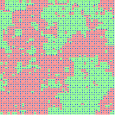
Fig. 5: By freezing the ferromagnet, it can happen that certain domains are showing up.
It is possible to get pictures like the one shown in fig. 5. Here, the so called Weiss domains are showing up in a very simple form. This is not guaranteed to happen since it hugely depends on the starting conditions (i.e., the distribution of spins when the lattice was generated). However, it is interesting that those domains can actually show up in simulation. The statistics that will be obtained will show up in the form of fig. 6.
Fig. 6: Statistic for a 32 x 32 lattice while going from beta = 0 to beta = 1.
At beta = 0.435 is the so called critical point of this model. This is where the phase transition actually occurs.
Points of Interest
The Ising model is quite a simple one that is cheap to simulate. It should be noted that it forms the basis for a lot of successful approaches in many scientific fields and can be extended in order to simulate completely different matters. The simulated annealing algorithm has also been built up on Monte-Carlo Ising simulations resulting in fast solutions of the traveling salesman problem and others.
The WebWorker will be a key technology for upcoming websites. It allows developers to let clients do intensive computations without resulting in an unresponsive website. Another key factor is that those computations can easily be canceled and controlled.
The simulation can be viewed live at http://html5.florian-rappl.de/Ising.
History
- v1.0.0 | Initial release | 29.01.2012
Florian lives in Munich, Germany. He started his programming career with Perl. After programming C/C++ for some years he discovered his favorite programming language C#. He did work at Siemens as a programmer until he decided to study Physics.
During his studies he worked as an IT consultant for various companies. After graduating with a PhD in theoretical particle Physics he is working as a senior technical consultant in the field of home automation and IoT.
Florian has been giving lectures in C#, HTML5 with CSS3 and JavaScript, software design, and other topics. He is regularly giving talks at user groups, conferences, and companies. He is actively contributing to open-source projects. Florian is the maintainer of AngleSharp, a completely managed browser engine.


 General
  News
News  Suggestion
  Question
  Bug
Bug  Answer
  Joke
Joke  Praise
  Rant
Rant  Admin
Admin 


 ). However, I think that the WebWorker is just an intermediate step (and gives us possibilities that are not possible in ECMAScript 3).