Visualization of High Dimensional Data using t-SNE with R

Introduction

One way to see and understand patterns from data is by means of visualization. In the space of AI, Data Mining, or Machine Learning, often knowledge is captured and represented in the form of high dimensional vector or matrix. This article will help you getting started with the t-SNE and Barnes-Hut-SNE techniques to visualize high-dimensional data/vector in R.

This article assumes that you have at least a basic expertise in R. Some useful references are provided at the end of the article. Please check [0] and [5] if you are not.

Background

R Environment

R is a language and environment for statistical computing and graphics. More about R, and installing R-packages can be read from [0] and [5].

There are several implementations of t-SNE out there [4] of which the t-SNE and Barnes-Hut-SNE implementations are available for use in R as tsne and Rtsne packages respectively.

What is t-SNE?

t-SNE was introduced by Laurens van der Maaten and Geoff Hinton in "Visualizing Data using t-SNE" [2]. t-SNE stands for t-Distributed Stochastic Neighbor Embedding. It visualizes high-dimensional data by giving each datapoint a location in a two or three-dimensional map. It is a variation of Stochastic Neighbor Embedding (Hinton and Roweis, 2002) that allows optimization, and produces significantly better visualizations by reducing the tendency to lump points together in the center of the map that often renders the visualization ineffective and unreadable. t-SNE is good at creating a map that reveals structure and embedding relationships at many different scales. This is particularly important for high-dimensional inter-related data that lie on several different low-dimensional manifolds, such as images of objects from multiple classes seen from multiple viewpoints.

The baseline version of t-SNE has O(N²) complexity. Later on, Maaten introduced the O(N log N) version of t-SNE a.k.a Barnes-Hut-SNE [3].

t-SNE will work with many form of high-dimensional data. Please check Maaten's FAQs [4] for answers to misc questions that you might have. The chance is that you will find answers to your questions there. In this article, we will demonstrate the use of t-SNE against the high-dimensional distributed word representation (also known as word embedding) produced by word2vec algorithm. This high-dimensional representation of words can be used in many natural language processing (NLP) applications.

Running t-SNE and Barnes-Hut-SNE in R

1. Download and install the tsne and Rtsne R-package.

See instruction for installing R-package. It is probably helpful to also look "R in action" text book to understand with the basic of datasets in R, loading data into R, and basic syntax of language covering the concept of variable, function, graph and using R-packages.

2. Obtain and import dataset to R.

You can use any high-dimensional vector data and import it into R. If you don't have one, I have provided a sample words embedding dataset produced by word2vec.

DISCLAIMER: The intention of sharing the data is to provide quick access so anyone can plot t-SNE immediately without having to generate the data themselves. The data produced does not necessarily reflect the quality of the technique as quality can be affected by many parameters and when we produced the word embedding we run the word2vec algorithm with all default parameters. The data is shared on an "AS IS" BASIS, WITHOUT WARRANTIES OR CONDITIONS OF ANY KIND, either express or implied. You need to agree to this before using the data.

The sample dataset can be downloaded here. To load the dataset into R, execute the following R command in R shell (assuming that the data is in d:\samplewordembedding.csv):

> mydata <- read.table("d:\\samplewordembedding.csv", header=TRUE, sep=",")

3. Copy the following R-script snippet and paste it into R command line.

The script below assumes that the input file is in d:\samplewordembedding.csv and the output plot files are generated in the root directory of drive d: d:\plot.0.jpg, d:\plot.1.jpg, etc. Be prepared that your CPU will spike a little bit and it will take several minutes to complete the tsne execution.

# loading data into R
mydata <- read.table("d:\\samplewordembedding.csv", header=TRUE, sep=",")

# load the tsne package
library(tsne)

# initialize counter to 0
x <- 0
epc <- function(x) {
    x <<- x + 1
    filename <- paste("d:\\plot", x, "jpg", sep=".")
    cat("> Plotting TSNE to ", filename, " ")

    # plot to d:\\plot.x.jpg file of 2400x1800 dimension
    jpeg(filename, width=2400, height=1800)

    plot(x, t='n', main="T-SNE")
    text(x, labels=rownames(mydata))
    dev.off()
}

# run tsne (maximum iterations:500, callback every 100 epochs, target dimension k=5)
tsne_data <- tsne(mydata, k=5, epoch_callback=epc, max_iter=500, epoch=100)

Similarly you can use Rtsne package, the faster O(n log n) Barnes-Hut-TSNE algorithm. Rtsne is an R wrapper of C++ Maatens' Barnes-Hut-TSNE written by jkrijthe. As you would expect, Rtsne completes much faster than tsne.

# load the Rtsne package
library(Rtsne)

# run Rtsne with default parameters
rtsne_out <- Rtsne(as.matrix(mydata))

# plot the output of Rtsne into d:\\barneshutplot.jpg file of 2400x1800 dimension
jpeg("d:\\barneshutplot.jpg", width=2400, height=1800)
plot(rtsne_out$Y, t='n', main="BarnesHutSNE")
text(rtsne_out$Y, labels=rownames(mydata))

Points of Interest

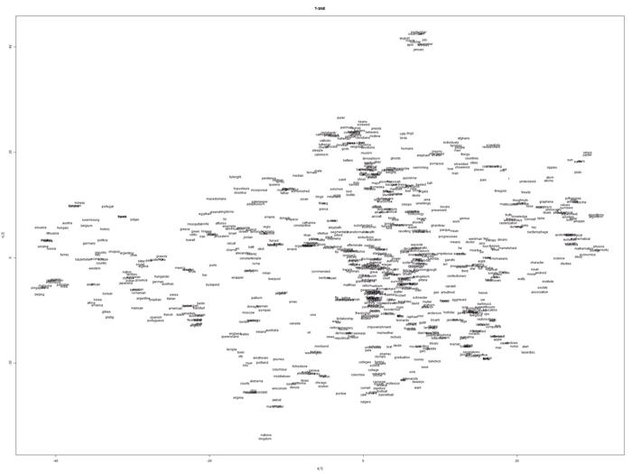
t-SNE separates and clusters group of words that we know semantically similar or different respectively. You can see from the plots, words about months of the years, countries, university/education related are clustered together. Based on my experience using the other techniques like kmeans and other common clustering tools available in R (e.g. kmeans, cluspot), applying to the same data, t-SNE reveals and informs us a much better insight in a cleaner and readable form of visualization.

It is an eye opening to be able to see through the powerful semantics produced by the t-SNE visualization from high-dimensional knowledge representation which otherwise would be just a set of floating numbers.

Below are the plots obtained from tsne & Rtsne.

TSNE plot:

Barnes-Hut-SNE plot:

We often appreciate things better when you are presented with the other options that are not as good. To give you something to compare, the following is a plot produced by the R-clusplot package including the R script to produce the plot. As you can see from the comparison, the plot produced by t-SNE and its variant is generally more readable by reducing the tendency to lump points together in the center of the map that often renders the visualization ineffective and unreadable.

# mydata is the matrix loaded into R previously. Run the following command if it isn't yet loaded into R. 
mydata <- read.table("d:\\samplewordembedding.csv", header=TRUE, sep=",")

# K-Means Clustering with 20 clusters
fit <- kmeans(mydata, 20)

# Cluster Plot against 1st 2 principal components
library(cluster) 
clusplot(mydata, fit$cluster, color=TRUE, shade=TRUE, labels=2, lines=0)

References

[0] About R

[1] Visualizing Data using t-SNE,  L. van der Maaten, G. Hinton, 2008

[2] Barnes-Hut-SNE, L. van der Maaten, 2013

[3] R-package TSNE

[4] Maaten T-SNE homepage

[5] Installing R and obtaining R-package

[6] word2vec algorithm

History

Initial version - version 1.0