Using Python to Solve Computational Physics Problems

Introduction

Laplace equation is a simple second-order partial differential equation. It is also a simplest example of elliptic partial differential equation. This equation is very important in science, especially in physics, because it describes behaviour of electric and gravitation potential, and also heat conduction. In thermodynamics (heat conduction), we call Laplace equation as steady-state heat equation or heat conduction equation.

In this article, we will solve the Laplace equation using numerical approach rather than analytical/calculus approach. When we say numerical approach, we refer to discretization. Discretization is a process to "transform" the continuous form of differential equation into a discrete form of differential equation; it also means that with discretization, we can transform the calculus problem into matrix algebra problem, which is favored by programming.

Here, we want to solve a simple heat conduction problem using finite difference method. We will use Python Programming Language, Numpy (numerical library for Python), and Matplotlib (library for plotting and visualizing data using Python) as the tools. We'll also see that we can write less code and do more with Python.

Background

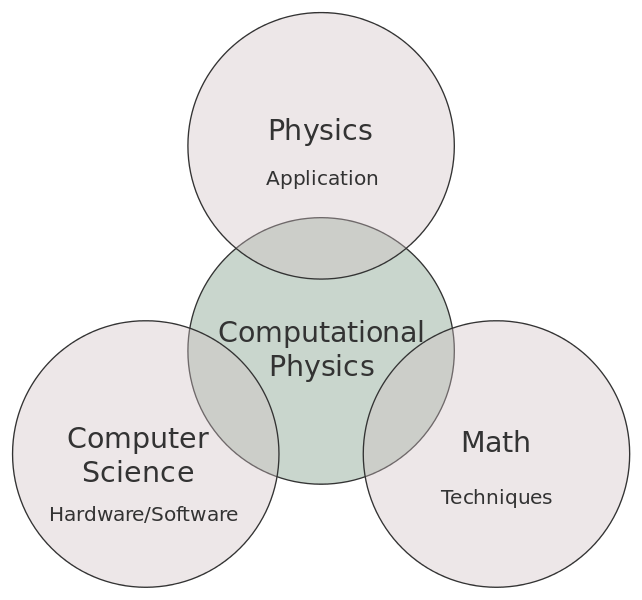
In computational physics, we "always" use programming to solve the problem, because computer program can calculate large and complex calculation "quickly". Computational physics can be represented as this diagram.

There are so many programming languages that are used today to solve many numerical problems, Matlab for example. But here, we will use Python, the "easy to learn" programming language, and of course, it's free. It also has powerful numerical, scientific, and data visualization library such as Numpy, Scipy, and Matplotlib. Python also provides parallel execution and we can run it in computer clusters.

Back to Laplace equation, we will solve a simple 2-D heat conduction problem using Python in the next section. Here, I assume the readers have basic knowledge of finite difference method, so I do not write the details behind finite difference method, details of discretization error, stability, consistency, convergence, and fastest/optimum iterating algorithm. We will skip many steps of computational formula here.

Instead of solving the problem with the numerical-analytical validation, we only demonstrate how to solve the problem using Python, Numpy, and Matplotlib, and of course, with a little bit of simplistic sense of computational physics, so the source code here makes sense to general readers who don't specialize in computational physics.

Preparation

To produce the result below, I use this environment:

• OS: Linux Ubuntu 14.04 LTS
• Python: Python 2.7
• Numpy: Numpy 1.10.4
• Matplotlib: Matplotlib 1.5.1

If you are running Ubuntu, you can use pip to install Numpy and Matplotib, or you can run this command in your terminal.

$ sudo apt-get install python-numpy

and use this command to install Matplotlib:

$ sudo apt-get install python-matplotlib

Note that Python is already installed in Ubuntu 14.04. To try Python, just type Python in your Terminal and press Enter.

You can also use Python, Numpy and Matplotlib in Windows OS, but I prefer to use Ubuntu instead.

Using the Code

This is the Laplace equation in 2-D cartesian coordinates (for heat equation):

Where T is temperature, x is x-dimension, and y is y-dimension. x and y are functions of position in Cartesian coordinates. If you are interested to see the analytical solution of the equation above, you can look it up here.

Here, we only need to solve 2-D form of the Laplace equation. The problem to solve is shown below:

What we will do is find the steady state temperature inside the 2-D plat (which also means the solution of Laplace equation) above with the given boundary conditions (temperature of the edge of the plat). Next, we will discretize the region of the plat, and divide it into meshgrid, and then we discretize the Laplace equation above with finite difference method. This is the discretized region of the plat.

We set Δx = Δy = 1 cm, and then make the grid as shown below:

Note that the green nodes are the nodes that we want to know the temperature there (the solution), and the white nodes are the boundary conditions (known temperature). Here is the discrete form of Laplace Equation above.

In our case, the final discrete equation is shown below.

Now, we are ready to solve the equation above. To solve this, we use "guess value" of interior grid (green nodes), here we set it to 30 degree Celsius (or we can set it 35 or other value), because we don't know the value inside the grid (of course, those are the values that we want to know). Then, we will iterate the equation until the difference between value before iteration and the value until iteration is "small enough", we call it convergence. In the process of iterating, the temperature value in the interior grid will adjust itself, it's "selfcorrecting", so when we set a guess value closer to its actual solution, the faster we get the "actual" solution.

We are ready for the source code. In order to use Numpy library, we need to import Numpy in our source code, and we also need to import Matplolib.Pyplot module to plot our solution. So the first step is to import necessary modules.

import numpy as np
import matplotlib.pyplot as plt

and then, we set the initial variables into our Python source code:

# Set maximum iteration
maxIter = 500

# Set Dimension and delta
lenX = lenY = 20 #we set it rectangular
delta = 1

# Boundary condition
Ttop = 100
Tbottom = 0
Tleft = 0
Tright = 0

# Initial guess of interior grid
Tguess = 30

What we will do next is to set the "plot window" and meshgrid. Here is the code:

# Set colour interpolation and colour map.
# You can try set it to 10, or 100 to see the difference
# You can also try: colourMap = plt.cm.coolwarm
colorinterpolation = 50
colourMap = plt.cm.jet

# Set meshgrid
X, Y = np.meshgrid(np.arange(0, lenX), np.arange(0, lenY))

np.meshgrid() creates the mesh grid for us (we use this to plot the solution), the first parameter is for the x-dimension, and the second parameter is for the y-dimension. We use np.arange() to arrange a 1-D array with element value that starts from some value to some value, in our case, it's from 0 to lenX and from 0 to lenY. Then we set the region: we define 2-D array, define the size and fill the array with guess value, then we set the boundary condition, look at the syntax of filling the array element for boundary condition above here.

# Set array size and set the interior value with Tguess
T = np.empty((lenX, lenY))
T.fill(Tguess)

# Set Boundary condition
T[(lenY-1):, :] = Ttop
T[:1, :] = Tbottom
T[:, (lenX-1):] = Tright
T[:, :1] = Tleft

Then we are ready to apply our final equation into Python code below. We iterate the equation using for loop.

# Iteration (We assume that the iteration is convergence in maxIter = 500)
print("Please wait for a moment")
for iteration in range(0, maxIter):
    for i in range(1, lenX-1, delta):
        for j in range(1, lenY-1, delta):
            T[i, j] = 0.25 * (T[i+1][j] + T[i-1][j] + T[i][j+1] + T[i][j-1])

print("Iteration finished")

You should be aware of the indentation of the code above, Python does not use bracket but it uses white space or indentation. Well, the main logic is finished. Next, we write code to plot the solution, using Matplotlib.

# Configure the contour
plt.title("Contour of Temperature")
plt.contourf(X, Y, T, colorinterpolation, cmap=colourMap)

# Set Colorbar
plt.colorbar()

# Show the result in the plot window
plt.show()

print("")

That's all, This is the complete code.

# Simple Numerical Laplace Equation Solution using Finite Difference Method
import numpy as np
import matplotlib.pyplot as plt

# Set maximum iteration
maxIter = 500

# Set Dimension and delta
lenX = lenY = 20 #we set it rectangular
delta = 1

# Boundary condition
Ttop = 100
Tbottom = 0
Tleft = 0
Tright = 30

# Initial guess of interior grid
Tguess = 30

# Set colour interpolation and colour map
colorinterpolation = 50
colourMap = plt.cm.jet #you can try: colourMap = plt.cm.coolwarm

# Set meshgrid
X, Y = np.meshgrid(np.arange(0, lenX), np.arange(0, lenY))

# Set array size and set the interior value with Tguess
T = np.empty((lenX, lenY))
T.fill(Tguess)

# Set Boundary condition
T[(lenY-1):, :] = Ttop
T[:1, :] = Tbottom
T[:, (lenX-1):] = Tright
T[:, :1] = Tleft

# Iteration (We assume that the iteration is convergence in maxIter = 500)
print("Please wait for a moment")
for iteration in range(0, maxIter):
    for i in range(1, lenX-1, delta):
        for j in range(1, lenY-1, delta):
            T[i, j] = 0.25 * (T[i+1][j] + T[i-1][j] + T[i][j+1] + T[i][j-1])

print("Iteration finished")

# Configure the contour
plt.title("Contour of Temperature")
plt.contourf(X, Y, T, colorinterpolation, cmap=colourMap)

# Set Colorbar
plt.colorbar()

# Show the result in the plot window
plt.show()

print("")

It's pretty short, huh? Okay, you can copy-paste and save the source code, name it findif.py. To execute the Python source code, open your Terminal, and go to the directory where you locate the source code, type:

$ python findif.py

and press Enter. Then the plot window will appear.

You can try to change the boundary condition's value, for example, you change the value of right edge temperature to 30 degree Celcius (Tright = 30), then the result will look like this:

Points of Interest

Python is an "easy to learn" and dynamically typed programming language, and it provides (open source) powerful library for computational physics or other scientific discipline. Since Python is an interpreted language, it's slow as compared to compiled languages like C or C++, but again, it's easy to learn. We can also write less code and do more with Python, so we don't struggle to program, and we can focus on what we want to solve.

In computational physics, with Numpy and also Scipy (numeric and scientific library for Python), we can solve many complex problems because it provides matrix solver (eigenvalue and eigenvector solver), linear algebra operation, as well as signal processing, Fourier transform, statistics, optimization, etc.

In addition to its use in computational physics, Python is also used in machine learning, even Google's TensorFlow uses Python.

History

• 21^st March, 2016: Initial version