Introduction
A set of pretty simple, but powerful functions was developed in R producing images of fractals. The two prime approaches are following: Kronecker product and IFS based (KPB and IFSB). In addition, a few algorithms were developed to produce different Brownian trees.
Description of the fractals in general and the mentioned above 3 categories are presented in [1-6].
My motivation is: to fulfill the absence of any decent fractal pictures in R on the Internet, particularly, related to these 3 categories. I was surprised when I found a few dozens of Brownian motions devoted articles/pictures in The R Journal [7], but none of Brownian tree picture. I think readers of CodeProject (CP) would be interested in it, because my intensive search using Google and R website confirmed: there is nothing essential realized/published on the Internet or in other sources regarding these types of fractals in R. Again, there are a lot of samples with code in C, C++, C#, VB, Python, etc., including a few online generators in JavaScript, but nothing in R.
It should be mentioned that all 3 approaches allow creating virtually infinite number of fractals. The only limitations would be the power of the used computer and creativity of the user.
In the online article [8] was presented a simple method to build fractals using a Kronecker product applied to a simple matrix that contains only zeros and ones. Author realized it in SAS/IML program, built and showed two fractals: Vicsek and "Landing at LaGuardia". The first fractal and many others realized in R would be shown in this article, including many original.
I already had a Barnsley fern fractal realized in PARI/GP and JavaScript [10-12]. But I ran at the article and the online IFS fractals generator [13] realized in JavaScript, which is able to produce more than 30 different fractals, including a Barnsley fern. This online tool is based on the generic approach of processing IFS tables [10], and this approach was realized in R. Again, it should be stressed, that I've used only the idea. The source code is not offered for download, but IFS tables are freely available. See samples of tables and description in [4,10,13].
To realize in R both KPB fractals and Brownian trees [9], - a set of plotting helper functions need to be created first. Such set was created in PARI/GP and later translated to R. The idea to use matrix filled with 0/1 was "re-invented" independently for building and plotting Brownian trees and other fractals in PARI/GP [11, 12], and it was not difficult to apply it to functions in R.
Plotting Helper Functions
It should be stressed that although any helper function is extremely useful, nevertheless, in many cases, it can't be applied, or it is just not as effective as simple direct plotting, E.g., look at pIfsFractal() function below, or at pVoronoiD() function in [14].
There are only 2 plotting helper functions: plotmat() and plotv2(), which are really generic plotting functions that were already used many times and proved their usefulness and reliability [12].
Let's take a closer look at these functions.
## R Helper Functions
#
## HFR#1 plotmat(): Simple plotting using matrix mat (filled with 0/nonzero int).
#  Where: mat - matrix; fn - file name (no extension); clr - color;
#         ttl - plot title; dflg - writing dump file flag (0-no/1-yes):
#         psz - picture size; cx - cex or scale.
plotmat <- function(mat, fn, clr, ttl, dflg=0, psz=600, cx=1.0) {
  m = nrow(mat); d = 0; X=NULL; Y=NULL;
  pf = paste0(fn, ".png"); df = paste0(fn, ".dmp");
  # Building X and Y arrays for plotting from not equal to zero values in mat.
  for (i in 1:m) {
    for (j in 1:m) {if(mat[i,j]==0){next} else {d=d+1; X[d]=i; Y[d]=j} }
  };
  cat(" *** Matrix(", m,"x",m,")", d, "DOTS\n");
  # Dumping if requested (dflg=1).
  if (dflg==1) {dump(c("X","Y"), df); cat(" *** Dump file:", df, "\n")};
  # Plotting
  if (ttl!="") {
    plot(X,Y, main=ttl, axes=FALSE, xlab="", ylab="", col=clr, pch=20, cex=cx)}
  else {par(mar=c(0,0,0,0));
    plot(X,Y, axes=FALSE, xlab=NULL, ylab=NULL, col=clr, pch=20, cex=cx)};
  # Writing png-file
  dev.copy(png, filename=pf, width=psz, height=psz);
  # Cleaning
  dev.off(); graphics.off();
}

## HFR#2 plotv2(): Simple plotting using 2 vectors (dumped into ".dmp" file).
# Where: fn - file name; clr - color; ttl - plot title; psz - picture size;
#        cx - cex or scale.
plotv2 <- function(fn, clr, ttl, psz=600, cx=1.0) {
  cat(" *** START:", date(), "clr=", clr, "psz=", psz, "\n");
  pf = paste0(fn, ".png"); df = paste0(fn, ".dmp");
  source(df); d = length(X);
  cat(" *** Plot file -", pf, "Source dump-file:", df, d, "DOTS\n");
  # Plotting
  if (ttl!="") {
    plot(X,Y, main=ttl, axes=FALSE, xlab="", ylab="", col=clr, pch=20, cex=cx)}
  else {par(mar=c(0,0,0,0));
    plot(X,Y, axes=FALSE, xlab=NULL, ylab=NULL, col=clr, pch=20, cex=cx)};
  # Writing png-file
  dev.copy(png, filename=pf, width=psz, height=psz);
  # Cleaning
  dev.off(); graphics.off();
  cat(" *** END:", date(), "\n");
}
First of all, they are very small, simple and clear. Each has less than 15 lines of code (without comments). So, it would be easy to translate them to another language.
The prime one is plotmat(). It was designed to handle plotting of the matrix filled with 0 and 1. Actually, in the current version, matrix could be filled with zeros and any other integer numbers.
This function has a few simple steps (see the code above):
- Using double "
for" loop to select points/dots with not equal to zero values from the mat matrix and build X and Y arrays for selected dots. These arrays later are used for dumping and plotting. - Writing a dump file if requested.
- Plotting X,Y dots.
- Saving a plot as a png-file.
Another function plotv2() is even simpler. It is plotting X,Y dots from a dump file created by the plotmat(). Also, it could be any similar dump file created by any function.
Requesting the plotmat() dump file is useful if the generating time is big. Having a dump file makes it easy and fast to repeat plotting with different colors, titles and sizes using the plotv2().
Usually, the generating time is big for the pIfsFractal() function and a Brownian tree related functions. The plotting time is big if the number of generated dots is huge.
Important remarks:
- All presented generating/plotting functions (except for the
pIfsFractal()) are using the plotmat() for the mat matrix. - In case of the re-plotting with the
plotv2(): 2 vectors X,Y are used from the dump file created by the plotmat(). - The file name used in the
plotmat() and plotv2() is without an extension (which will be added as ".png" and ".dmp" when needed).
Kronecker Product Based Approach to Generating Fractals
The origin and nature of Kronecker product based fractals is explained in more details in [3].
Let's take a closer look at the following 2 functions:
## Kronecker power of a matrix.
## Where: m - initial matrix, n - power.
matkronpow <- function(m, n) {
  if (n<2) {return (m)};
  r = m; n = n-1;
  for(i in 1:n) {r = r%x%m};
  return (r);
}

## Generate and plot Kronecker product based fractals.
## gpKronFractal(m, n, pf, clr, ttl, dflg, psz, cx):
## Where: m - initial matrix (filled with 0/int); n - order of the fractal;
## fn - plot file name (without extension); clr - color; ttl - plot title;
## dflg - writing dump file flag (0/1); psz - picture size; cx - cex.
gpKronFractal <- function(m, n, fn, clr, ttl, dflg=0, psz=640, cx=1.0) {
  fign="Kpbf";
  cat(" *** START:", date(), "n=", n, "clr=", clr, "psz=", psz, "\n");
  if(fn=="") {fn=paste0(fign,"o", n)} else {fn=paste0(fn)};
  if(ttl!="") {ttl=paste0(ttl,", order ", n)};
  cat(" *** Plot file -", fn, "title:", ttl, "\n");
  r = matkronpow(m, n);
  plotmat(r, fn, clr, ttl, dflg, psz, cx);
  cat(" *** END:", date(), "\n");
}
As you can see, they are very simple and clear. The matkronpow(m, n) returns m x m x m ... (n times product). The second function, actually, has only 2 lines of code for generating and plotting, and all other statements are just for the logging.
TIP: Create and use any kind of helper functions. This will help to keep the code of other functions small, clear and stable.
What possibly needs to be explained within a function having 5-10 lines of R code?
Samples of Designing/Plotting Kronecker Product Based Fractals
Designing Kronecker product based fractals is easy using simple text presentation of the initial matrix. In this case, it is very clear what a designed matrix is representing. Well, not always. Especially, if the initial matrix was created using a few steps of applying manipulation with many different matrices.
Note: The KPBFdesign.html page from [3] could be very handy.
To show how to design/plot a KPB fractal, - the new "O" fractal was chosen. There are the following 3 easy steps for this "O" fractal.
1. The Basic Matrix Design
Use simple text presentation like the following:
Prime matrix   or   Inverted matrix (0 and 1 are swaped)
1111111                   0000000
1000001                   0111110
1011101                   0100010
1011101                   0100010
1011101                   0100010
1000001                   0111110
1111111                   0000000
2. "Translate" it to the 1-2 Rows of the R Code as follows
M <- matrix(c(1,1,1,1,1,1,1, 1,0,0,0,0,0,1, 1,0,1,1,1,0,1, 1,0,1,1,1,0,1,
 1,0,1,1,1,0,1, 1,0,0,0,0,0,1, 1,1,1,1,1,1,1), ncol=7, nrow=7, byrow=TRUE);
3. Execute it in the R GUI Window
gpKronFractal(M, 3, "OF3t", "maroon", "'O' fractal");
Another design approach would be to create an initial matrix using the Kronecker product of 2 different matrices and applying the gpKronFractal() to it.
Here is such a sample:
M <- matrix(c(0,1,0, 1,1,1, 0,1,0), ncol=3, nrow=3, byrow=TRUE);
M1 <- matrix(c(1,0,1, 0,1,0, 1,0,1), ncol=3, nrow=3, byrow=TRUE);
R=M%x%M1;
gpKronFractal(R, 2, "Crosses2F", "maroon", "2 crosses based fractal", 1);
Important remarks:
- The generating function
gpKronFractal() is using an initial matrix M to build a resultant matrix and plot it. - Try setting a low n first, because a big n would require a lot of memory and time.
Here is the code for testing Vicsek, Sierpinski carpet, Rug and "T" fractals:
M <- matrix(c(0,1,0, 1,1,1, 0,1,0), ncol=3, nrow=3, byrow=TRUE);
gpKronFractal(M, 4, "VicsekFractal1","red", "Vicsek Fractal");

M <- matrix(c(1,1,1, 1,0,1, 1,1,1), ncol=3, nrow=3, byrow=TRUE);
gpKronFractal(M, 4, "SierpinskiCF1", "maroon", "Sierpinski carpet fractal");

M <- matrix(c(1,1,1,1,1, 1,0,0,0,1, 1,0,0,0,1, 1,0,0,0,1, 1,1,1,1,1),
 ncol=5, nrow=5, byrow=TRUE);
gpKronFractal(M, 4, "RugF", "brown", "Rug fractal", 1);

M <- matrix(c(1,1,1,1,1, 1,1,1,0,1, 1,0,0,0,1, 1,1,1,0,1, 1,1,1,1,1),
 ncol=5, nrow=5, byrow=TRUE);
gpKronFractal(M,4,"GPFRT","darkviolet","",1,600);
Note: If your computer is not a super fast one, then it could take very long time. Use a dump flag = 1, to save the generated fractal for a re-plotting.
Remark: On the other hand, while testing "T" fractal on the old laptop with WinXP, I got very strange results: using the gpKronFractal() was 6 times faster than using the plotv2(). I think, it happened because of low memory causing a memory swapping process.
See it for yourself below in the snippets and their output logs.
M = matrix(c(1,1,1,1,1, 1,1,1,0,1, 1,0,0,0,1, 1,1,1,0,1, 1,1,1,1,1),ncol=5,nrow=5,byrow=T);
gpKronFractal(M,4,"GPFRT","darkviolet","",1,600,0.5);
 *** START: Thu Jun 08 16:57:12 2017 n= 4 clr= darkviolet psz= 600
 *** Plot file - GPFRT title:
 *** Matrix( 625 x 625 ) 160000 DOTS
 *** Dump file: GPFRT.dmp
 *** END: Thu Jun 08 16:59:08 2017

plotv2("GPFRT", "maroon", "'T' fractal", 640, 0.5);
 *** START: Thu Jun 08 17:00:31 2017 clr= maroon psz= 640
 *** Plot file - GPFRT.png Source dump-file: GPFRT.dmp 160000 DOTS
 *** END: Thu Jun 08 17:12:58 2017
And I need to stress it again: applications of fractals, also, time of the execution evaluation or measuring is out of my interests.
TIP: Test the speed of generating/plotting on your computer and choose the best function for you.
You can use shown above 2 samples "as is" for such testing.
All four resultant fractals are presented below in the Figure 1 - Figure 4.
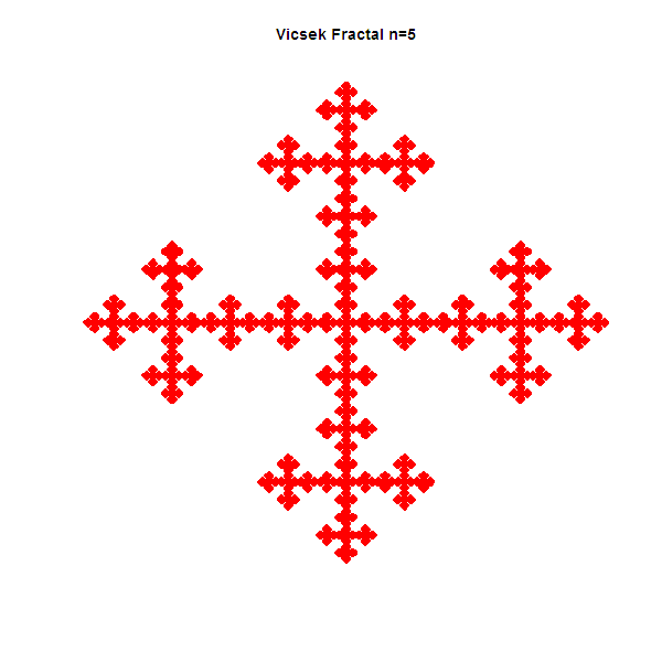

Figures 1-4: Vicsek, Sierpinski carpet, Rug and "T" fractals
TIP: Right-click and save any figure above to see a much bigger image.
TRICK: "T" fractal above looks like having order 3, because only 3 sizes of "T" are present. To see that this is actually the order 4 fractal, it should be plotted differently:
M <- matrix(c(1,1,1,1,1, 1,1,1,0,1, 1,0,0,0,1, 1,1,1,0,1, 1,1,1,1,1),
 ncol=5,nrow=5,byrow=T);
gpKronFractal(M,4,"GPFRT2","darkviolet","",0, 1280, 0.5);
# Note: bigger size + scaling are requested.
In addition, it should be zoomed in, e.g., using Microsoft Office Picture Manager. Only now all 4 sizes of "T" are visible.
The New Version of R Scripts
The new version of R scripts (related mostly to the KPBF plotting) was upgraded in many ways. Now the plotmat() function is executing faster, consuming less memory, dealing with rotation, supporting background color and has a few other improvements.
Testing shows that now, in many cases, it is more appropriate to re-plot fractal with the plotmat() function than using a dump file.
The plotv2() function is still useful if the generating time is big. E.g., for Brownian trees plotting.
IFS Based Approach to Generating Fractals
Only one function realizes IFS based approach. Let's take a closer look at this function.
## Plotting fractals using IFS style
## Plotting is based on already calculated M x 7 table of coefficients
## in the input file.
## Note: 1. Input ifs-file should be dat-file; output is set as png-file.
##       2. Swap 2nd and 3rd column if you've got data used in Java,
##          JavaScript, etc.

## pIfsFractal(fn, n, clr, ttl, psz, cx): Plot fractals using IFS style.
## Where: fn - file name; n - number of dots; clr - color; ttl - plot title,
##        psz - plot size, cx - cex.

pIfsFractal <- function(fn, n, clr, ttl, psz=600, cx=0.5) {
  # pf - plot file name; df - data/ifs file name;
  pf=paste0(fn,".png"); df=paste0(fn,".dat");
  cat(" *** IFSSTART:", date(), "n=", n, "clr=", clr, "psz=", psz, "\n");

  # Reading a complete data table from the file: space delimited, no header.
  # Table has any number of rows, but always 7 columns is a must.
  (Tb = as.matrix(read.table(df, header=FALSE)))
  tr = nrow(Tb)
  # Creating matrix M1 from 1st 4 columns of each row.
  M1 = vector("list",tr);
  for (i in 1:tr) {M1[[i]] = matrix(c(Tb[i,1:4]),nrow=2)}
  # Creating matrix M2 from columns 5,6 of each row.
  M2 = vector("list",tr);
  for (i in 1:tr) {M2[[i]] = matrix(c(Tb[i,5:6]),nrow=2)}
  ## Creating matrix M3 (actually a vector) from column 7 of each row.
  M3 = c(Tb[1:tr,7])

  x = numeric(n); y = numeric(n);
  x[1] = y[1] = 0;

  # Main loop
  for (i in 1:(n-1)) {
    k = sample(1:tr, prob=M3, size=1);
    M = as.matrix(M1[[k]]);
    z = M%*%c(x[i],y[i]) + M2[[k]];
    x[i+1] = z[1];
    y[i+1] = z[2];
  }
  # Plotting
  if (ttl!="") {
    plot(x,y, main=ttl, axes=FALSE, xlab="", ylab="", col=clr, pch=20, cex=cx)}
  else {par(mar=c(0,0,0,0));
    plot(x,y, axes=FALSE, xlab=NULL, ylab=NULL, col=clr, pch=20, cex=cx)};
  # Writing png-file
  dev.copy(png, filename=pf,width=psz,height=psz);
  # Cleaning
  dev.off(); graphics.off();
  cat(" *** IFS  END:", date(), "\n");
}
The code above is well commented and doesn't need an additional explanation, but look in [10] for the description of an algorithm, tables and a computer generation.
Important remarks:
- The generation is based on an already calculated m x 7 table of coefficients [10] in the input file.
- An input ifs-file should be the dat-file (find samples in the downloaded zip-file); an output is set as a png-file.
- Swap the 2nd and the 3rd columns of the Ifs-table if you've got data used in Java, JavaScript, etc.
Testing Generation/Plotting for a Few Fractals
Note: Related data files are presented in GPFRdatafiles.txt file and in GPRFDATA folder.
pIfsFractal("BarnsleyFern", 100000, "dark green", "Barnsley fern fractal", ,0.25);

pIfsFractal("Pentaflake", 100000, "blue", "Pentaflake fractal");

pIfsFractal("Sierpinski3", 100000, "red", "Sierpinski triangle fractal");

pIfsFractal("TriangleF", 100000, "maroon", "Triangle fractal");
All four resultant fractals are presented below in the Figure 5 - Figure 8.
Figures 5-8: Barnsley fern, Pentaflake, Sierpinski triangle and Triangle fractals
Generating Brownian Tree Fractals
All four functions generating Brownian tree fractals were translated from PARI/GP [11, 12]. But, in turn, PARI/GP functions were translated from other languages. And this fact proves that the basic algorithm in each function is correct.
Let's take a closer look at one of these functions.
# ALL 4 versions are in GFIRALLfuncs.R
# translation of PARI/GP: http:
# Generate and plot Brownian tree. Version #1.
# gpBrownianTree1(m, n, clr, fn, ttl, dflg)
# Where: m - defines matrix m x m; n - limit of the number of moves;
# fn - file name (.ext will be added); ttl - plot title; dflg - 0-no dump,
# 1-dump.
gpBrownianTree1 <- function(m, n, clr, fn, ttl, dflg=0) {
cat(" *** START:", date(),"m=",m,"n=",n,"clr=",clr,"\n");
M = matrix(c(0),ncol=m,nrow=m,byrow=T);
# Seed in center
x = m%/%2; y = m%/%2;
M[x,y]=1;
pf=paste0(fn,".png");
cat(" *** Plot file -",pf,"\n");
# Main loops: Generating matrix M
for (i in 1:n) {
if(i>1) {
x = sample(1:m, 1, replace=F)
y = sample(1:m, 1, replace=F)}
while(1) {
ox=x; oy=y;
x = x + sample(-1:1, 1, replace=F);
y = y + sample(-1:1, 1, replace=F);
if(x<=m && y<=m && x>0 && y>0 && M[x,y])
{if(ox<=m && oy<=m && ox>0 && oy>0){M[ox,oy]=1; break}}
if(!(x<=m && y<=m && x>0 && y>0)) {break}
}
}
plotmat(M, fn, clr, ttl, dflg); ## Plotting matrix M
cat(" *** END:",date(),"\n");
}
#gpBrownianTree1(400,15000,"red", "BT13", "Brownian Tree v.1-1",1); ## Dump (Seed in center alwys now)
The other 3 functions find in the GFIRALLfuncs.R file.
All four functions have similar 3 steps:
- Setting an initial "seed" point/dot (predefined or random).
- Simulating a "random walk" using different, but always just 2 loops: "
for" and "while". The important parts within this second step are:
- to make a random "walking step" to the closest free space
- to ensure that each "walking step" is within the matrix
- to save a successful "walking step" location in the matrix
- Plotting resultant matrix representing a Brownian Tree.
Important remarks:
- All plotting functions are using the
plotmat(). - Because "random walks" are used to fill the resultant matrix, - each time a differently looking tree will be produced by all 4 functions (even for the same number of requested dots and matrix sizes).
Testing Generation/Plotting for Brownian Tree v.1 - v.4
gpBrownianTree1(400,15000,"red", "BTv1", "Brownian Tree v.1", 1);

gpBrownianTree2(400,5000,"brown", "BTv2", "Brownian Tree v.2", 1);

gpBrownianTree3(400,5000,"dark green", "BTv31", "Brownian Tree v.3-1", 1);

gpBrownianTree4(400,15000,"navy", "BTv41", "Brownian Tree v.4-1", 1);
All four versions of Brownian tree fractals are presented below in the Figure 9 - Figure 12.
Figures 9-12: Brownian tree fractals v.1 - v.4
If you need a different language, in the [9] find samples of Brownian trees in 47 langauges.
Conclusion
It should be stressed again: this project demonstrates the technique of plotting for 3 types of fractals in the R language. The same types of fractals can be found in many other languages [3,8,9,11,12], but not in the R.
Presented 3 approaches to generating fractals (together with the set of support functions) can produce virtually infinite number of fractals. Really, there is an infinite number of matrices (that could be used in the KPB approach), also an infinite number of initial data tables (that could be used in the IFSB approach). Not to mention infinite Brownian trees.
The real limitation is only a power of the used computer, and, of course, creativity of the new fractal designer.
In the files, GPFRsamples.txt and v2Samples.txt, many additional testing samples are provided for all 3 types of fractals to keep you busy and enjoying new fractals.
Note: All KPBF samples in GPFRsamples.txt file can be used "as is" with the new version.
References
- Fractal, Wikipedia, the free encyclopedia, URL: https://en.wikipedia.org/wiki/Fractal
- Kronecker product, Wikipedia, the free encyclopedia, URL: https://en.wikipedia.org/wiki/Kronecker_product.
- Voevudko, A.E. (2017) Generating Kronecker Product Based Fractals. Code Project.
- Iterated function system, Wikipedia, the free encyclopedia, URL: https://en.wikipedia.org/wiki/Iterated_function_system
- Brownian tree, Wikipedia, the free encyclopedia, URL: https://en.wikipedia.org/wiki/Brownian_tree
- Diffusion-limited aggregation, Wikipedia, the free encyclopedia, URL: https://en.wikipedia.org/wiki/Diffusion-limited_aggregation
- The R Journal, URL: https://journal.r-project.org/
- Wicklin R. (2014), Self-similar structures from Kronecker products, URL: http://blogs.sas.com/content/iml/2014/12/17/self-similar-structures-from-kronecker-products.html
- Brownian tree, Rosetta Code Wiki, URL: http://rosettacode.org/wiki/Brownian_tree
- Barnsley fern, Wikipedia, the free encyclopedia, URL: https://en.wikipedia.org/wiki/Barnsley_fern
- Voevudko, A.E., User page, OEIS Wiki, URL: http://oeis.org/wiki/User:Anatoly_E._Voevudko
- Voevudko, A.E., User page, Rosetta Code Wiki, URL: http://rosettacode.org/wiki/User:AnatolV
- Toal R., Iterated Function Systems, URL: http://cs.lmu.edu/~ray/notes/ifs/
- Voevudko, A.E. (2017) Generating Random Voronoi Diagrams. Code Project
History
- 04/17/2018 -- Adding code file with upgraded version of
plotmat(), plotv2(), etc., and file with new samples. A lot of minor editing: mostly changing "look & feel". Fixing a few typos. Adding "History" chapter and "New version of R scripts" sub-chapter. - 07/05/2017 -- Initial posting
I've started programming in a machine code and an assembly language for IBM 370 mainframe, and later programmed in many other languages, including, of course, C/C++/C# and ASP/ASP.net/VB.net.
I've created many system automation tools and websites for companies and universities.
In addition, I've always been a scientist interested in Computer Science, NT, AI, etc.
Now I'm using mainly scripting languages for NT small problems and computer graphics.


