Introduction
In this article, we will cover self driving car methodology using the Udacity Open sourced Self driving car simulator. Here, we will cover how self driving car is implemented and this can be easily extended to different scenarios. This includes enacting of how self driving car is implemented using Behavioural Cloning. The process includes Deep Neural Network, feature extraction with Convolution network as well as continuous regression.
The Entire Process
We will drive the car in training track inside a simulator. As we drive the car through the simulator, we are going to be taking images at each instances of the drive.
The images we take will be representing the training dataset and the label for each specific image will be the steering angle of the car at that specific instance.
We will show all of these images to convolution neural network and allow it to learn and how to drive it autonomously as the behaviour of the manual driver. The main variable that our model will learn to adjust is the steering angle of the car at any given instance. It will effectively adjust to learn to appropriate degree based on the situation that it finds itself.
The behavioural cloning technique is very useful and plays a big role in real life self driving cars as well.
Collection of Data
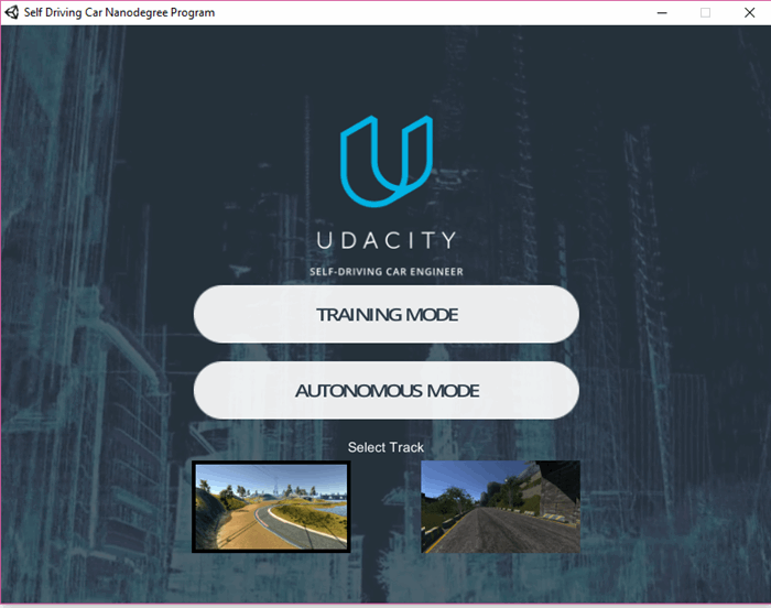
We will first download the simulator to start our behavioural training process.
We will be starting by driving the car in simulator using keyboard keys. With that, we will be able to train convolution neural network to monitor the controlled operation and movement of the vehicle. And depending on how we are driving, it will be copied to autonomous mode using our behaviour, hence the term behavioural cloning (watching the behaviour and copying the data that we are providing it, how well the neural network works is determined by how will we be able to drive the car ourselves for driving skills and then into the neural network.
We will download the simulator from the following link:
Once we have mastered how the car driven controls in simulator using keyboard keys, then we get started with record button to collect data.

We will save the data from it in a specified folder.
We will take data from 3 laps of simulated driving. We will get to know how we drive the car. The tracks are structured on the same to challenge the neural network to overcome sharp terms.
As we drive through the whole track, we realize that different parts of the track have different textures, different curvatures, layouts and landscapes. All of these are different features extracted by neural networks. We will try to drive the car along the center, it is a regression based approach.
We will also go in reverse laps to capture more data to generalize.
As the simulated environment is doing the reverse lap, we balance between both left and right direction avoiding bias.
Developing Machine learning algorithms works with trying different sets of data until it reaches the intended target and so by analysing the loss and accuracy plot. Detrming that our model is overfitting or underfitting and then adjusting it accordingly.
We will see that it is a regression type example since the error metrics is mean squared error. If the mean squared error is high in both training and validation, then we will be dealing with underfitting problem, otherwise if the mean squared is low on the training but high on the validation, then our model will be overfitting
Our motto for the simulator would be to focus simply on driving straight and at the middle all the times, 3 laps forward and then backwards.
For the simulator, the car is equipped with 3 cameras, one each at the left, center and right. Each camera records a footage for each image it collects a value for the steering angle, brake, throttle at the current image.
The Training Process
For the process of getting the self driving car working, we have to upload the images that we recorded using the simulator.
First of all, we will open GITHUB. We will open it up in a web browser.
If we do not have an account, we will create a new one. With that, we will create a new repo as shown in the figure below:
We name the repository with a given name and keep it public.
We will now open a command window and see if git is installed.
If not, we will have to install git.
Now we will go to the folder where we have saved the recording which contains image and the csv files.
We will issue a command:
Git init
Then again, we use:
Git add .
and the folder will be replicated accordingly.
We will be using Google Colab for doing the training process.
We will open a new python3 notebook and get started. Next, we will git clone the repo.
!git clone https://github.com/AbhiLegend/SDCE
We will now import all the libraries needed for training process. It will use Tensorflow backend and keras at frontend.
import os
import numpy as np
import matplotlib.pyplot as plt
import matplotlib.image as mpimg
import keras
from keras.models import Sequential
from keras.optimizers import Adam
from keras.layers import Convolution2D, MaxPooling2D, Dropout, Flatten, Dense
from sklearn.utils import shuffle
from sklearn.model_selection import train_test_split
from imgaug import augmenters as iaa
import cv2
import pandas as pd
import ntpath
import random
We wil use datadir as the name given to the folder itself and take the parameters itself. Using head, we will show the first five values for the CSV on the desired format.
datadir = 'SDCE'
columns = ['center', 'left', 'right', 'steering', 'throttle', 'reverse', 'speed']
data = pd.read_csv(os.path.join(datadir, 'driving_log.csv'), names = columns)
pd.set_option('display.max_colwidth', -1)
data.head()
As this is picking up the entire path from the local machine, we need to use ntpath function to get the network path assigned. We will declare a name path_leaf and assign accordingly.
    def path_leaf(path):
  head, tail = ntpath.split(path)
  return tail
data['center'] = data['center'].apply(path_leaf)
data['left'] = data['left'].apply(path_leaf)
data['right'] = data['right'].apply(path_leaf)
data.head()
We will bin the number of values where the number will be equal to 25 (odd number aimed to get center distribution). We will see the histogram using the np.histogram option on data frame ‘steering’, we will divide it to the number of bins.
    num_bins = 25
samples_per_bin = 400
hist, bins = np.histogram(data['steering'], num_bins)
center = (bins[:-1]+ bins[1:]) * 0.5
plt.bar(center, hist, width=0.05)
plt.plot((np.min(data['steering']), np.max(data['steering'])), \
(samples_per_bin, samples_per_bin))
We keep samples at 400 and then we draw a line. We see the data is centered along the middle that is 0.
We wil specify a variable rove_list = []
We will specify samples we want to remove using looping construct through every single bin we will iterate through all the steering data. We will shuffle the data and romve some from it as it is now uniformly structured after shuffling.The output will be the distribution of steering angle that are much more uniform. There are significant amount of left steering angle and right steering angle eliminating the bias to drive straight all the time.
    print('total data:', len(data))
remove_list = []
for j in range(num_bins):
  list_ = []
  for i in range(len(data['steering'])):
    if data['steering'][i] >= bins[j] and data['steering'][i] <= bins[j+1]:
      list_.append(i)
  list_ = shuffle(list_)
  list_ = list_[samples_per_bin:]
  remove_list.extend(list_)

print('removed:', len(remove_list))
data.drop(data.index[remove_list], inplace=True)
print('remaining:', len(data))

hist, _ = np.histogram(data['steering'], (num_bins))
plt.bar(center, hist, width=0.05)
plt.plot((np.min(data['steering']), np.max(data['steering'])), \
(samples_per_bin, samples_per_bin))
We will now load the image into array to manipulate them accordingly. We will define a function named locd_img_steering. We will have image path as empty list and steering as empty list and then loop through. We use iloc selector as data frame based on the specific index we will use cut data for now.
print(data.iloc[1])
def load_img_steering(datadir, df):
image_path = []
steering = []
for i in range(len(data)):
indexed_data = data.iloc[i]
center, left, right = indexed_data[0], indexed_data[1], indexed_data[2]
image_path.append(os.path.join(datadir, center.strip()))
steering.append(float(indexed_data[3]))
image_path.append(os.path.join(datadir,left.strip()))
steering.append(float(indexed_data[3])+0.15)
image_path.append(os.path.join(datadir,right.strip()))
steering.append(float(indexed_data[3])-0.15)
image_paths = np.asarray(image_path)
steerings = np.asarray(steering)
return image_paths, steerings
image_paths, steerings = load_img_steering(datadir + '/IMG', data)
    X_train, X_valid, y_train, y_valid = train_test_split(image_paths, steerings, \
test_size=0.2, random_state=6)
print('Training Samples: {}\nValid Samples: {}'.format(len(X_train), len(X_valid)))
We will be splitting the image path as well as storing arrays accordingly.
We will have the histograms now.
    fig, axes = plt.subplots(1, 2, figsize=(12, 4))
axes[0].hist(y_train, bins=num_bins, width=0.05, color='blue')
axes[0].set_title('Training set')
axes[1].hist(y_valid, bins=num_bins, width=0.05, color='red')
axes[1].set_title('Validation set')
In the next steps, we normalize the data and in the nvdia model, we will have to keep it in a UAV pattern as well as slice unnecessary information. We preprocess the image too.
    def zoom(image):
  zoom = iaa.Affine(scale=(1, 1.3))
  image = zoom.augment_image(image)
  return image
image = image_paths[random.randint(0, 1000)]
original_image = mpimg.imread(image)
zoomed_image = zoom(original_image)

fig, axs = plt.subplots(1, 2, figsize=(15, 10))
fig.tight_layout()

axs[0].imshow(original_image)
axs[0].set_title('Original Image')

axs[1].imshow(zoomed_image)
axs[1].set_title('Zoomed Image')

def pan(image):
  pan = iaa.Affine(translate_percent= {"x" : (-0.1, 0.1), "y": (-0.1, 0.1)})
  image = pan.augment_image(image)
  return image
image = image_paths[random.randint(0, 1000)]
original_image = mpimg.imread(image)
panned_image = pan(original_image)

fig, axs = plt.subplots(1, 2, figsize=(15, 10))
fig.tight_layout()

axs[0].imshow(original_image)
axs[0].set_title('Original Image')

axs[1].imshow(panned_image)
axs[1].set_title('Panned Image')
def img_random_brightness(image):
    brightness = iaa.Multiply((0.2, 1.2))
    image = brightness.augment_image(image)
    return image
image = image_paths[random.randint(0, 1000)]
original_image = mpimg.imread(image)
brightness_altered_image = img_random_brightness(original_image)

fig, axs = plt.subplots(1, 2, figsize=(15, 10))
fig.tight_layout()

axs[0].imshow(original_image)
axs[0].set_title('Original Image')

axs[1].imshow(brightness_altered_image)
axs[1].set_title('Brightness altered image ')

def img_random_flip(image, steering_angle):
    image = cv2.flip(image,1)
    steering_angle = -steering_angle
    return image, steering_angle
random_index = random.randint(0, 1000)
image = image_paths[random_index]
steering_angle = steerings[random_index]

original_image = mpimg.imread(image)
flipped_image, flipped_steering_angle = img_random_flip(original_image, steering_angle)

fig, axs = plt.subplots(1, 2, figsize=(15, 10))
fig.tight_layout()

axs[0].imshow(original_image)
axs[0].set_title('Original Image - ' + 'Steering Angle:' + str(steering_angle))

axs[1].imshow(flipped_image)
axs[1].set_title('Flipped Image - ' + 'Steering Angle:' + str(flipped_steering_angle))
def random_augment(image, steering_angle):
    image = mpimg.imread(image)
    if np.random.rand() < 0.5:
      image = pan(image)
    if np.random.rand() < 0.5:
      image = zoom(image)
    if np.random.rand() < 0.5:
      image = img_random_brightness(image)
    if np.random.rand() < 0.5:
      image, steering_angle = img_random_flip(image, steering_angle)

    return image, steering_angle
ncol = 2
nrow = 10

fig, axs = plt.subplots(nrow, ncol, figsize=(15, 50))
fig.tight_layout()

for i in range(10):
  randnum = random.randint(0, len(image_paths) - 1)
  random_image = image_paths[randnum]
  random_steering = steerings[randnum]

  original_image = mpimg.imread(random_image)
  augmented_image, steering = random_augment(random_image, random_steering)

  axs[i][0].imshow(original_image)
  axs[i][0].set_title("Original Image")

  axs[i][1].imshow(augmented_image)
  axs[i][1].set_title("Augmented Image")

def img_preprocess(img):
    img = img[60:135,:,:]
    img = cv2.cvtColor(img, cv2.COLOR_RGB2YUV)
    img = cv2.GaussianBlur(img,  (3, 3), 0)
    img = cv2.resize(img, (200, 66))
    img = img/255
    return img
image = image_paths[100]
original_image = mpimg.imread(image)
preprocessed_image = img_preprocess(original_image)

fig, axs = plt.subplots(1, 2, figsize=(15, 10))
fig.tight_layout()
axs[0].imshow(original_image)
axs[0].set_title('Original Image')
axs[1].imshow(preprocessed_image)
axs[1].set_title('Preprocessed Image')
def batch_generator(image_paths, steering_ang, batch_size, istraining):

  while True:
    batch_img = []
    batch_steering = []

    for i in range(batch_size):
      random_index = random.randint(0, len(image_paths) - 1)

      if istraining:
        im, steering = random_augment(image_paths[random_index], steering_ang[random_index])

      else:
        im = mpimg.imread(image_paths[random_index])
        steering = steering_ang[random_index]

      im = img_preprocess(im)
      batch_img.append(im)
      batch_steering.append(steering)
    yield (np.asarray(batch_img), np.asarray(batch_steering))
We will design our Model architecture. We have to classify the traffic signs too that's why we need to shift from Lenet 5 model to NVDIA model. With behavioural cloning, our dataset is much more complex then any dataset we have used.
We are dealing with images that have (200,66) dimensions.
Our current datset has 3511 images to train with but MNSIT has around 60,000 images to train with.’
Our behavioural cloning code has simply has to return appropriate steering angle which is a regression type example.
For these things, we need a more advanced model which is provided by nvdia and known as nvdia model.
The architecture of nvdia model is as shown below:
For defining the model architecture, we need to define the model object.
Normalization state can be skipped as we have already normalized it.
We will add the convolution layer.
As compared to the model, we will organize accordingly.
The Nvdia model uses 24 filters in the layer along with a kernel of size 5,5.
We will introduce sub sampling. The function reflects to stride length of the kernel as it processes through an image, we have large images.
Horizontal movement with 2 pixels at a time, similarly vertical movement to 2 pixels at a time.
As this is the first layer, we have to define input shape of the model too i.e., (66,200,3) and the last function is an activation function that is “elu”.
    def nvidia_model():
  model = Sequential()
  model.add(Convolution2D(24, 5, 5, subsample=(2, 2), \
            input_shape=(66, 200, 3), activation='elu'))
Revisting the model, we see that our second layer has 36 filters with kernel size (5,5) same subsampling option with stride length of (2,2) and conclude this layer with activation ‘elu’.
model.add(Convolution2D(36, 5, 5, subsample=(2, 2), activation='elu'))
According to Nvdia model, it shows we have 3 more layers in the convolutional neural network. With 48 filters, with 64 filters (3,3) kernel 64 filters (3,3) kernel Dimensions have been reduced significantly so for that we will remove subsampling from 4th and 5th layer.
    model.add(Convolution2D(64, 3, 3, activation='elu'))
model.add(Convolution2D(64, 3, 3, activation='elu'))
Next we add a flatten layer. We will take the output array from previous convolution neural network to convert it into a one dimensional array so that it can be fed to fully connected layer to follow:
model.add(Flatten())
Our last convolution layer outputs an array shape of (1,18) by 64.
model.add(Convolution2D(64, 3, 3, activation='elu'))
We end the architecture of Nvdia model with a dense layer containing a single output node which will output the predicted steering angle for our self driving car. Now we will use model.compile() to compile our architecture as this is a regression type example the metrics that we will be using will be mean squared error and optimize as Adam. We will be using relatively a low learning rate that it can help on accuracy. We will use dropout layer to avoid overfitting the data. Dropout Layer sets the input of random fraction of nodes to “0” during each update. During this, we will generate the training data as it is forced to use a variety of combination of nodes to learn from the same data. We will have to separate the convolution layer from fully connected layer with a factor of 0.5 is added so it converts 50 percent of the input to 0. We Will define the model by calling the nvdia model itself. Now we will have the model training process.To define training parameters, we will use model.fit(), we will import our training data X_Train, training data ->y_train, we have less data on the datasets we will require more epochs to be effective. We will use validation data and then use Batch size.
def nvidia_model():
model = Sequential()
model.add(Convolution2D(24, 5, 5, subsample=(2, 2), \
input_shape=(66, 200, 3), activation='elu'))
model.add(Convolution2D(36, 5, 5, subsample=(2, 2), activation='elu'))
model.add(Convolution2D(48, 5, 5, subsample=(2, 2), activation='elu'))
model.add(Convolution2D(64, 3, 3, activation='elu'))
model.add(Convolution2D(64, 3, 3, activation='elu'))
model.add(Flatten())
model.add(Dense(100, activation = 'elu'))
model.add(Dense(50, activation = 'elu'))
model.add(Dense(10, activation = 'elu'))
model.add(Dense(1))
optimizer = Adam(lr=1e-3)
model.compile(loss='mse', optimizer=optimizer)
return model
model = nvidia_model()
print(model.summary())
history = model.fit_generator(batch_generator(X_train, y_train, 100, 1),
                                  steps_per_epoch=300,
                                  epochs=10,
                                  validation_data=batch_generator(X_valid, y_valid, 100, 0),
                                  validation_steps=200,
                                  verbose=1,
                                  shuffle = 1)
Why We Use ELU Over RELU
We can have dead relu this is when a node in neural network essentially dies and only feeds a value of zero to nodes which follows it. We will change from relu to elu. Elu function has always a chance to recover and fix it errors means it is in a process of learning and contributing to the model. We will plot the model and then save it accordingly in h5 format for a keras file.
    plt.plot(history.history['loss'])
plt.plot(history.history['val_loss'])
plt.legend(['training', 'validation'])
plt.title('Loss')
plt.xlabel('Epoch')
We will save the model:
model.save('model.h5')
Then download the model itself.
    from google.colab import files
files.download('model.h5')
The Connection Part
This step is required to run the model in the simulated car.
For implementing web service using python, we need to install flask. We will use Anaconda environment. Flask is a python micro framework that is used to build the web app.
We will use Visual Studio code for the use.
We will open the folder where we kept the saved *.h5 file, then again open a file but before that, we will install some dependencies.
We will also create an anaoconda environment too for doing our work.
F:\SDCE>conda create --name myenviron
Fetching package metadata ...............
Solving package specifications:
Package plan for installation in environment C:\Users\abhis\Miniconda3\envs\myenviron:
Proceed ([y]/n)? y
We will activate the environment:
    F:\SDCE>activate myenviron

(myenviron) F:\SDCE>
Now we will install the dependencies for web sockets:
---------------------------------------------------------------------------------
(myenviron) F:\SDCE>conda install -c anaconda flask
Fetching package metadata .................
Solving package specifications: .
Warning: 4 possible package resolutions (only showing differing packages):
- anaconda::jinja2-2.10-py36_0, anaconda::vc-14.1-h21ff451_3
- anaconda::jinja2-2.10-py36_0, anaconda::vc-14.1-h0510ff6_3
- anaconda::jinja2-2.10-py36h292fed1_0, anaconda::vc-14.1-h21ff451_3
- anaconda::jinja2-2.10-py36h292fed1_0, anaconda::vc-14.1-h0510ff6_3
Package plan for installation in environment C:\Users\abhis\Miniconda3\envs\myenviron:
The following NEW packages will be INSTALLED:
click: 7.0-py36_0 anaconda
flask: 1.0.2-py36_1 anaconda
itsdangerous: 1.1.0-py36_0 anaconda
jinja2: 2.10-py36_0 anaconda
markupsafe: 1.1.0-py36he774522_0 anaconda
pip: 18.1-py36_0 anaconda
python: 3.6.7-h33f27b4_1 anaconda
setuptools: 27.2.0-py36_1 anaconda
vc: 14.1-h21ff451_3 anaconda
vs2015_runtime: 15.5.2-3 anaconda
werkzeug: 0.14.1-py36_0 anaconda
wheel: 0.32.3-py36_0 anaconda
Proceed ([y]/n)? y
vs2015_runtime 100% |
vc-14.1-h21ff4 100% |
python-3.6.7-h 100% |
click-7.0-py36 100% |
itsdangerous-1 100% |
markupsafe-1.1 100% |
setuptools-27. 100% |
werkzeug-0.14. 100% |
jinja2-2.10-py 100% |
wheel-0.32.3-p 100% |
flask-1.0.2-py 100% |
pip-18.1-py36_ 100% |
Now we will write a python file, first import Flask. From flask, we can initialize our application as app and set it equal to flask. We have an instance for web app. We will declare a special variable known as name which will suffice on main. We will define a function greeting which will return a string welcome. Then we can specify a router decorator @app.route(/home) which is going on the URL home invokes the following function returns the appropriate String as shown in the browser. We will run the python code and now we have a web app that has some content returned by python. We will install some more dependencies such as socketio and others so that we can connect the Self driving car autonomous mode and using web sockets to make it work using the trained keras model file.
(myenviron) F:\SDCE1>conda install -c conda-forge eventlet
Fetching package metadata ...............
Solving package specifications: .
Package plan for installation in environment C:\Users\abhis\Miniconda3\envs\myenviron:
The following NEW packages will be INSTALLED:
ca-certificates: 2018.11.29-ha4d7672_0 conda-forge
cffi: 1.11.5-py36hfa6e2cd_1001 conda-forge
cryptography: 1.7.1-py36_0
eventlet: 0.23.0-py36_1000 conda-forge
greenlet: 0.4.13-py36_0 conda-forge
idna: 2.8-py36_1000 conda-forge
openssl: 1.0.2p-hfa6e2cd_1001 conda-forge
pyasn1: 0.4.4-py_1 conda-forge
pycparser: 2.19-py_0 conda-forge
pyopenssl: 16.2.0-py36_0 conda-forge
six: 1.12.0-py36_1000 conda-forge
Proceed ([y]/n)? y
ca-certificate 100% |
openssl-1.0.2p 100% |
greenlet-0.4.1 100% |
idna-2.8-py36_ 100% |
pyasn1-0.4.4-p 100% |
pycparser-2.19 100% |
six-1.12.0-py3 100% |
cffi-1.11.5-py 100% |
pyopenssl-16.2 100% |
eventlet-0.23. 100% |
(myenviron) F:\SDCE1>
------conda package sockets
(myenviron) F:\SDCE1>conda install -c conda-forge python-socketio
Fetching package metadata ...............
Solving package specifications: .
Package plan for installation in environment C:\Users\abhis\Miniconda3\envs\myenviron:
The following NEW packages will be INSTALLED:
python-engineio: 3.0.0-py_0 conda-forge
python-socketio: 2.1.2-py_0 conda-forge
Proceed ([y]/n)? y
python-enginei 100% |
python-socketi 100% |
Within the myenviron, we will run the drive.py file and connect to the local server. We then run the simulator in autonomous mode and when connection is established, we see the self driving car moving in the environment.
import socketio
import eventlet
import numpy as np
from flask import Flask
from keras.models import load_model
import base64
from io import BytesIO
from PIL import Image
import cv2
sio = socketio.Server()
app = Flask(__name__)
speed_limit = 10
def img_preprocess(img):
img = img[60:135,:,:]
img = cv2.cvtColor(img, cv2.COLOR_RGB2YUV)
img = cv2.GaussianBlur(img, (3, 3), 0)
img = cv2.resize(img, (200, 66))
img = img/255
return img
@sio.on('telemetry')
def telemetry(sid, data):
speed = float(data['speed'])
image = Image.open(BytesIO(base64.b64decode(data['image'])))
image = np.asarray(image)
image = img_preprocess(image)
image = np.array([image])
steering_angle = float(model.predict(image))
throttle = 1.0 - speed/speed_limit
print('{} {} {}'.format(steering_angle, throttle, speed))
send_control(steering_angle, throttle)
@sio.on('connect')
def connect(sid, environ):
print('Connected')
send_control(0, 0)
def send_control(steering_angle, throttle):
sio.emit('steer', data = {
'steering_angle': steering_angle.__str__(),
'throttle': throttle.__str__()
})
if __name__ == '__main__':
model = load_model('model.h5')
app = socketio.Middleware(sio, app)
eventlet.wsgi.server(eventlet.listen(('', 4567)), app)
The Self driving car simulator as when on running mode:
Conclusion
The entire solution step by step is included in the ipython file. Feel free to tweak it. I have also shared all steps needed to follow along the tutorial.
History
I am into software Development for less than a year and i have participated in 2 contests here at Codeproject:-Intel App Innovation Contest 2012 and Windows Azure Developer Challenge and been finalist at App Innovation contest App Submission award winner as well won two spot prizes for Azure Developer Challenge.I am also a finalist at Intel Perceptual Challenge Stage 2 with 6 entries nominated.I also won 2nd prize for Ultrabook article contest from CodeProject
Link:-
http://www.codeproject.com/Articles/523105/Ultrabook-Development-My-Way
Microsoft MVA Fast Track Challenge Global Winner.
Ocutag App Challenge 2013 Finalist.
My work at Intel AppUp Store:-
UltraSensors:-
http://www.appup.com/app-details/ultrasensors
UltraKnowHow:-
http://www.appup.com/app-details/ultraknowhow


 General
  News
News  Suggestion
  Question
  Bug
Bug  Answer
  Joke
Joke  Praise
  Rant
Rant  Admin
Admin 


