Numerical Laplace Transforms and Inverse Transforms in C#

• Download demo - 5.18 KB
• Download source - 10.9 KB

Contents

• Introduction
• Why Laplace Transforms?
• The Inverse Laplace Transform
• The Laplace Transform
• Comments
• References

Introduction

In modeling many physical processes described by differential or partial differential equations, solutions can be obtained analytically using Laplace transforms. For most of the more interesting problems, however, inverting the solution is often a problem. Additionally, there are other classes of problems where manipulation of Laplace transforms is simple, but the function of interest is not easily transformed. This article presents a C# implementation of the Stehfest algorithm for Laplace transform inversion as well as an algorithm to compute the Laplace transform integral, numerically, for an arbitrary function.

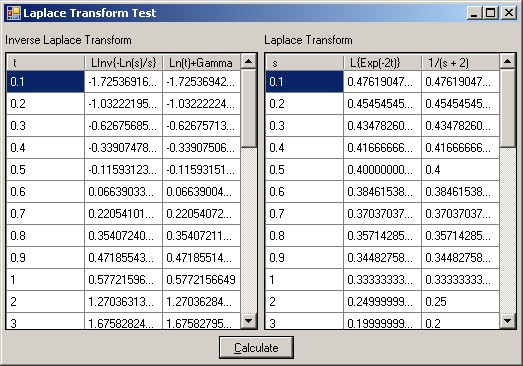
The source code and a test program for checking the Laplace transform calculations are available from the links above. A screenshot of the test program is shown below.

Why Laplace Transforms?

Many physical processes are described by the diffusion equation including temperature distributions, diffusion of chemicals, and fluid flow in porous media. My particular interest is in modeling oil reservoirs, so the diffusion or diffusivity equation is of fundamental importance. In cases where a reservoir can be considered uniform and homogeneous, the time variable in the partial differential equation can be transformed using Laplace transforms, eliminating the time derivatives, and converting a partial differential equation into an ordinary differential equation, which is fairly easily solved. Problems involving Laplace transforms also arise in computing statistical functions and other areas of math.

For reference, the diffusivity equation used for radial flow of a single fluid near a well in a homogeneous reservoir can be written as follows, where p_D represents the dimensionless pressure, r_D represents the dimensionless radial distance from a well, and t_D represents dimensionless time. To actually solve the equation is beyond the scope of this article; however, a suitable boundary and initial conditions are needed, and the result is typically the Laplace transform of the pressure distribution in an oil reservoir. For anyone interested in oil field applications, please see the classic paper by Van Everdingen and Hurst.

In other cases, we may already know the solution of the equation for some ideal situation, for example, when the flow from a well is constant. In the real world, however, things are rarely constant, and to determine the actual solution, it is necessary to calculate the convolution of the ideal solution with a boundary condition that varies as a function of time. In Laplace transforms, that simply involves multiplying the Laplace transforms of two functions, but again, the result is the Laplace transform of the desired solution, and we need to convert that back to real values. For reference, the convolution consists of an integral, expressed as follows:

In addition, there are cases where an ideal solution cannot be determined explicitly using Laplace transforms, but requires the use of finite difference approximations or other numerical techniques, for example, to account for some strange geometry, irregular boundaries, or other strangeness. In these cases, we might have the basic solution in terms of some tabulated results or a fitted curve, and then need to calculate the convolution to adjust for variations not included in the numerical model. Note that in complex cases, calculating the basic solution may take hours of computer time, so running a new finite difference calculation isn't an option, especially if we need to display interactive graphics. An example of this is in the paper by Fair (1981).

A Laplace transform is an integral transform. The transform and the corresponding inverse transform are defined as follows:

A complete description of the transforms and inverse transforms is beyond the scope of this article. Anyone needing more information can refer to the "bible" of numerical mathematics, Abramowitz and Stegun (1970). A fairly complete tabulation of analytical Laplace transforms is also included.

Since the most common programming problem involves taking inverse Laplace transforms, I'll discuss that first, then tackle the problem of numerically calculating the Laplace transform integral.

The Inverse Laplace Transform

As you can see from the equation defining the inverse Laplace transform, direct calculation using brute force is formidable, because it involves calculating a complex path integral. Fortunately, there are some efficient numerical methods available for computing the inverse transform. Of these methods, one of the best was presented by Harald Stehfest (1970) and has become known as the Stehfest Algorithm. The algorithm itself is documented in the reference, but contains a typographical error that was later corrected. Stehfest points out that the algorithm requires an even number of coefficients, and is limited to functions that do not oscillate rapidly and that have no discontinuities. Fortunately, solutions to many practical equations rarely suffer from those problems. A web page [^] maintained by Dr. Peter Valko also shows some other algorithms that may be useful, especially when the Stehfest Algorithm cannot be applied. The equations used for the Stehfest Algorithm for Laplace transform inversion are as follows:

My implementation of the Stehfest Algorithm is fairly straightforward. Since the coefficients, V_i, do not depend on the function to be inverted, they can all be calculated once before doing any inversions. The C# code is shown below.

class Laplace 
{ 
    const int DefaultStehfest = 14; 
    public delegate double FunctionDelegate(double t); 
    static double[] V; // Stehfest coefficients 
    static double ln2; // log of 2
 
    public static void InitStehfest(int N) 
    { 
        ln2 = Math.Log(2.0); 
        int N2 = N / 2; 
        int NV = 2 * N2; 
        V = new double[NV]; 
        int sign = 1; 
        if ((N2 % 2) != 0) 
            sign = -1; 
        for (int i = 0; i < NV; i++) 
        { 
            int kmin = (i + 2) / 2; 
            int kmax = i + 1; 
            if (kmax > N2) 
                kmax = N2; 
            V[i] = 0; 
            sign = -sign; 
            for (int k = kmin; k <= kmax; k++) 
            { 
                V[i] = V[i] + (Math.Pow(k, N2) / Factorial(k)) * (Factorial(2 * k) 
                     / Factorial(2 * k - i - 1)) / Factorial(N2 - k) 
                     / Factorial(k - 1) / Factorial(i + 1 - k); 
            } 
            V[i] = sign * V[i]; 
        } 
    }
 
    public static double InverseTransform(FunctionDelegate f, double t) 
    { 
        double ln2t = ln2 / t; 
        double x = 0; 
        double y = 0; 
        for (int i = 0; i < V.Length; i++) 
        { 
            x += ln2t; 
            y += V[i] * f(x); 
        } 
        return ln2t * y; 
    } 

    public static double Factorial(int N) 
    { 
        double x = 1; 
        if (N > 1) 
        { 
            for (int i = 2; i <= N; i++) 
                x = i * x; 
        } 
        return x; 
    } 
}

I've found that a default of N = 14 coefficients gives reasonable results in C#, but depending on the hardware you use and the specific functions being inverted, more or less coefficients may yield better accuracy. Stehfest notes that the optimum number of coefficients mainly depends on the number of digits used in the floating point calculations, and above a certain limit, the numerical truncation errors start to swamp any increase in accuracy. For the test project, N = 14 yields between 7 and 8 decimal digits of precision.

To implement the inverse Laplace transform, I defined a static class Laplace. The static constructor calculates the default number of Stehfest coefficients the first time the class is referenced. Private static members of the class are used to save the Stehfest coefficients, V, and also the value of Ln(2) to avoid having to recalculate it every time. In case it's necessary to change the number of coefficients at run time, the InitStehfest(int N) method can be called to recalculate. Note that there is also a Factorial(int N) method included, since that is needed to calculate the Stehfest coefficients.

The function containing the Laplace transform is defined as a delegate, so that it can be passed as a parameter to the InverseTransform(FunctionDelegate f, double t) method that calculates the inverse transform at the specified value of t. As an example of using the transform inversion, the following code snippet defines a Laplace transform function equal to Ln(s)/s, then calculates the inverse transform at a value of t = 2.

double f(double s)
{
    return -Math.Log(s)/s;
}
 ...
double LinvCalc = Laplace.InverseTransform(f, 2.0);

The Laplace Transform

To calculate the Laplace transform of a function, it's necessary to calculate the Laplace integral defined above. The main problems involved lie in two areas:

1. the integral has an upper limit of infinity and
2. the exponential function inside the integral requires special consideration if accuracy is to be maintained.

Since directly calculating infinite integrals is impossible on a finite computer, the first "trick" I use is to change the Laplace transform integral into an equivalent finite integral by substituting u = e^-t. Using this variable transformation, when t = 0, u = 1 and when t approaches infinity, u approaches 0. This is shown in the following equations:

Essentially, what I've done is map the interval between 0 and infinity onto the interval between 0 and 1, thereby avoiding having to deal with infinity. If you take a close look at the equation, though, you'll note that there's still a potential problem, since it requires evaluating Ln(u = 0) and also u^{(s - 1)} when u = 0. If s < 1, there's also the possibility of a singularity. Fortunately, evaluating Ln(u = 0) isn't a real problem, since if the Laplace transform exists, the limiting value at t = infinity or u = 0 must be exactly 0. The problem with a singularity for s < 1 may, however, still be a problem. Evaluating Laplace transforms at small values of s, corresponding to infinite times, is a notoriously difficult problem that I've chosen to ignore, since I rarely need to work with such small values of s.

My implementation of the transform calculation is fairly straightforward. As shown in the following code, I added a double Transform(FunctionDelegate F, double s) method that calculates the integral using the supplied function, F, at the specified value of the Laplace parameter, s. The formula Math.Pow(u, s - 1) * F(-Math.Log(u)) corresponds to the transformed integral kernel, and u is the independent variable. The while loop implements Simpson's Rule[^] to calculate the integral, but for efficiency, I've written the algorithm using du as half of the interval usually shown in standard Simpson's rule formulas. This allowed me to factor a 2 out of the loop, and multiply once at the end, rather than every loop iteration. When you're dealing with large loops and trying to maintain precision, every little bit helps.

public static double Transform(FunctionDelegate F, double s)
{
    const int DefaultIntegralN = 5000;
    double du = 0.5 / (double)DefaultIntegralN;
    double y =  - F(0) / 2.0;
    double u = 0;
    double limit = 1.0 - 1e-10;
    while (u < limit)
    {
        u += du;
        y += 2.0 * Math.Pow(u, s - 1) * F(-Math.Log(u));
        u += du;
        y += Math.Pow(u, s - 1) * F(-Math.Log(u));
    }
    return 2.0 * y * du / 3.0;
}

Note also that I've set the loop limit to 1.0 - 1e-10, rather than 1.0. When dealing with a sum of small numbers, numerical precision can haunt you, so I've learned to never count on the sums of floating point numbers being exactly equal to anything.

Using the Laplace transform method is simple. Simply define a function that returns a value, given a value of the variable, t, then call the Transform method to retrieve the Laplace transform for any given value of the Laplace variable, s. The following code snippet shows how to compute the Laplace transform of the function e^-2t for a Laplace variable value of s = 2.

double F(double t)
{
    return 1.0 / Math.Exp(2.0*t);
}
 ...
double LCalc = Laplace.Transform(F, 2);

After running some tests, I concluded that 5000 intervals in the Simpson's Rule calculation are enough to ensure good precision. If you play with this algorithm, you may want to check that. In the case of "strange" functions, you may need to use more divisions to avoid losing precision. Conversely, you may be able to use fewer intervals and gain some speed. For the test case shown in the example program, 5000 integral divisions yield around 9 or 10 decimal digits of precision.

Comments

I hope these algorithms will be of interest to someone and keep them from having to reinvent the wheel. Using analytical solutions to physical problems is still often a viable method, even though the current trend is to move more towards finite difference methods. Analytical solutions, however, are often orders of magnitude faster and more accurate. An example of a commercial application using these techniques can be seen on my website[^].

If anyone has any ideas for improving the performance and flexibility of the algorithms presented in this article, I'd be very pleased to hear about them. Specifically, there could be improvements when calculating the Laplace transforms of functions with singularities and discontinuities, although those aren't usually associated with physical processes.

To me, it's interesting to see how things have changed over the years. I originally implemented these algorithms back before there were PCs, and a Laplace transform inversion took about 10 minutes on a TI-99 programmable calculator. Later, the same algorithms were coded in Turbo Pascal 1.0, and would run in less than a minute on an 8086. Now, I run thousands per second on my laptop. To be fair, though, I have to point out that the main improvements have come by optimizing the functions, since many of the problems of interest to me involve Modified Bessel functions. As a point of reference, engineers who worked on the calculations presented in the Van Everdingen and Hirst paper have told me that to compute the functions tabulated in the paper, they had a bank of over a dozen secretaries armed with tables of mathematical functions and mechanical calculators, and they could turn out about one column in the tables per day. In comparison, I now turn out the equivalent of one column in a few milliseconds.

If those were the good old days, no thank you!

References

• Van Everdingen, A. F. and W. Hurst, "The Application of the Laplace Transformation to Flow Problems in Reservoirs," Trans., AIME (194) 186, 305-324.
• Fair, Walter B. Jr., "Pressure Buildup Analysis with Wellbore Phase Redistribution," SPEJ (April 1981), 259-270.
• Abramowitz, Milton, and Irene Stegun, Handbook of Mathematical Functions, National Bureau of Standards, Washington, 1970.
• Stehfest, H., "Algorithm 368 - Numerical Inversion of Laplace Transforms," Communications of the ACM, (1970) 13, 47.
• Valko, Peter, Texas A&M University.