Applied Mathematics in C# via the Extreme Numerical Libraries for .NET

Introduction

In algebra, a polynomial is normally expressed as a function of x (of an n^th order) and plots its points to form a curvilinear path. A curvilinear graph normally implies continuity; that is, every point that comprises the curve has a tangent line. This means that at every point, there is a change in direction. This is sometimes called a differential coefficient. Because the tangent line is rarely horizontal, it would have a slope. Suppose we download the Extreme Numerical Libraries for .NET to reference the DLLs. You can download this numerical math library at http://www.extremeoptimization.com. It is basically a collection of DLLs that define classes that contain the methods and data members for most types of numerical computations. This library installs itself in the Program Files directory: therefore, when referencing the appropriate DLLs, you right-click the references button in the Solution Explorer. You then go to browse, and locate the DLL, which resides in the bin subdirectory. The reference choice depends on the type of numerical computation. This can range from differential equations to vector operations. Now having done that, we can then write a program that gives us all of the information needed to, say, find its roots. The code will construct a polynomial and then perform operations that provide the needed corresponding information. Here is a polynomial: x^4 - 10x^3 + 35x^2 - 50x + 24. Consider this code:

using System;
using Extreme.Mathematics.Curves;
public class Program
 {
   public static void Main(string[] args)
    {
     int index;
     Polynomial polynomial1 = new Polynomial(3);
     polynomial1[3] = 1;
     polynomial1[2] = 1;
     polynomial1[1] = 0;
     polynomial1[0] = -2
     double[] coefficients = new double[] {-2, 0, 1, 1};
     Polynomial polynomial2 = new Polynomial(coefficients);
     double[] roots = new double[] {1, 2, 3, 4};
     Polynomial polynomial3 = Polynomial.FromRoots(roots);
            
     double[] xValues = new double[] {1, 2, 3, 4};
     double[] yValues = new double[] {1, 4, 10, 8};

      Polynomial polynomial4 =  Polynomial.GetInterpolatingPolynomial(xValues, yValues);

      Console.WriteLine("polynomial3 = {0}", polynomial3.ToString());
      Console.WriteLine("polynomial1.Parameters.Count = {0}", 
                polynomial1.Parameters.Count);
      Console.Write("polynomial1 parameters:");
    for(index = 0; index < polynomial1.Parameters.Count; index++)
      Console.Write("{0} ", polynomial1.Parameters[index]);
      Console.WriteLine();
            
      Console.Write("polynomial2 parameters:");
    for(index = 0; index < polynomial2.Parameters.Count; index++)
      Console.Write("{0} ", polynomial2.Parameters[index]);
      Console.WriteLine();
      polynomial2.Parameters[0] = 1;
      polynomial2[0] = 1;
            
      Console.WriteLine("Degree of polynomial3 = {0}", polynomial3.Degree);
            
      Console.WriteLine("polynomial1.ValueAt(2) = {0}", polynomial1.ValueAt(2));
            
      Console.WriteLine("polynomial1.SlopeAt(2) = {0}", polynomial1.SlopeAt(2));
            
      Curve derivative = polynomial1.GetDerivative();
      Console.WriteLine("Slope at 2 (derivative) = {0}", derivative.ValueAt(2));
            
      Console.WriteLine("Type of derivative: {0}",
        derivative.GetType().FullName);
      Console.Write("Derivative parameters: ");
      for(index = 0; index < derivative.Parameters.Count; index++)
      Console.Write("{0} ", derivative.Parameters[index]);
      Console.WriteLine();
            
      Console.WriteLine("Type of derivative for polynomial3: {0}", 
                polynomial3.GetDerivative().GetType().FullName);
            
    Line tangent = polynomial1.TangentAt(2);
    Console.WriteLine("Tangent line at 2:");
    Console.WriteLine("  Y-intercept = {0}", tangent.Parameters[0]);
    Console.WriteLine("  Slope = {0}", tangent.Parameters[1]);

            
    Console.WriteLine("Integral of polynomial1 between 0 and 1 = {0}",
                polynomial1.Integral(0, 1));
               roots = polynomial1.FindRoots();
    Console.WriteLine("Number of roots of polynomial1: {0}",
                roots.Length);
    Console.WriteLine("Value of root 1 = {0}", roots[0]);
        
    roots = polynomial3.FindRoots();
    Console.WriteLine("Number of roots of polynomial3: {0}",
                roots.Length);
    Console.WriteLine("Value of root = {0}", roots[0]);
    Console.WriteLine("Value of root = {0}", roots[1]);
            
    Console.WriteLine("Value of root = {0}", roots[2]);
    Console.WriteLine("Value of root = {0}", roots[3]);
             Console.Write("Press Enter key to exit...");
    Console.ReadLine();
        }
    } 

Here is the output of the compilation. Note that this code was run as a Console Application project in Visual C# 2010 express. Prior to running this code, right-click the references, go to browse, and add the Extreme.Mathematics.Curves DLL:

polynomial3 = x^4-10x^3+35x^2-50x+24
polynomial1.Parameters.Count = 4
polynomial1 parameters:-2 0 1 1
polynomial2 parameters:-2 0 1 1
Degree of polynomial3 = 4
polynomial1.ValueAt(2) = 10
polynomial1.SlopeAt(2) = 16
Slope at 2 (derivative) = 16
Type of derivative: Extreme.Mathematics.Curves.Quadratic
Derivative parameters: 0 2 3 0
Type of derivative for polynomial3: Extreme.Mathematics.Curves.Polynomial
Tangent line at 2:
  Y-intercept = -22
  Slope = 16
Integral of polynomial1 between 0 and 1 = -1.41666666666667
Number of roots of polynomial1: 1
Value of root 1 = 1
Number of roots of polynomial3: 4
Value of root = 1
Value of root = 2
Value of root = 2.99999999999999
Value of root = 4.00000000000001

In certain types of engineering, an x y graph refers to the horizontal axis as the axis of reals and the vertical axis as the axis of the imaginaries. i^2 = -1. this is an imaginary number that is used, and often demonstrates vector paths. An example of a complex number is a = 2 + 4i. Now if b = 1 – 3i, c = -3, and d = 1 + 1.73205080756888i, we can then perform operations using these complex numbers with the aim of attaining the trigonometric, exponential, logarithmic, and hyperbolic functions of them. Consider this code:

using System;
using Extreme.Mathematics;
public class Program 
{
      public static void Main(string[] args)
      {            
    Console.WriteLine("DoubleComplex.Zero = {0}", DoubleComplex.Zero);
              Console.WriteLine("DoubleComplex.One = {0}", DoubleComplex.One);
    // The imaginary unit is given by DoubleComplex.I:
    Console.WriteLine("DoubleComplex.I = {0}", DoubleComplex.I);
    Console.WriteLine();

    //
    // Construct some complex numbers
    //
    // Real and imaginary parts:
    //   a = 2 + 4i
    DoubleComplex a = new DoubleComplex(2, 4);
    Console.WriteLine("a = {0}", a);
    //   b = 1 - 3i
    DoubleComplex b = new DoubleComplex(1, -3);
    Console.WriteLine("b = {0}", b.ToString());
    // From a real number:
    //   c = -3 + 0i
    DoubleComplex c = new DoubleComplex(-3);
    Console.WriteLine("c = {0}", c.ToString());
    // Polar form:
    //   d = 2 (cos(Pi/3) + i sin(Pi/3))
    DoubleComplex d = DoubleComplex.FromPolar(2, Constants.Pi/3);
    
    Console.WriteLine("d = {0}", d);
               Console.WriteLine();

    //
    // Parts of complex numbers
    //
    Console.WriteLine("Parts of a = {0}:", a);
    Console.WriteLine("Real part of a = {0}", a.Re);
    Console.WriteLine("Imaginary part of a = {0}", a.Im);
    Console.WriteLine("Modulus of a = {0}", a.Modulus);
    Console.WriteLine("Argument of a = {0}", a.Argument);
    Console.WriteLine();

    //
    // Basic arithmetic:
    //
    Console.WriteLine("Basic arithmetic:");
    DoubleComplex e = -a;
    Console.WriteLine("-a = {0}", e);
    e = a + b;
    Console.WriteLine("a + b = {0}", e);
    e = a - b;
    Console.WriteLine("a - b = {0}", e);
    e = a * b;
    Console.WriteLine("a * b = {0}", e);
    e = a / b;
    Console.WriteLine("a / b = {0}", e);
    // The conjugate of a complex number corresponds to
    // the "Conjugate" method:
    e = a.Conjugate();
    Console.WriteLine("Conjugate(a) = ~a = {0}", e);
    Console.WriteLine();

    //
    // Functions of complex numbers
    //
    // Most of these have corresponding static methods 
    // in the System.Math class, but are extended to complex 
    // arguments.
    Console.WriteLine("Functions of complex numbers:");

    // Exponentials and logarithms
    Console.WriteLine("Exponentials and logarithms:");
    e = DoubleComplex.Exp(a);
    Console.WriteLine("Exp(a) = {0}", e);
    e = DoubleComplex.Log(a);
    Console.WriteLine("Log(a) = {0}", e);
    e = DoubleComplex.Log10(a);
    Console.WriteLine("Log10(a) = {0}", e);
    // You can get a point on the unit circle by calling
    // the ExpI method:
    e = DoubleComplex.ExpI(2*Constants.Pi/3);
    Console.WriteLine("ExpI(2*Pi/3) = {0}", e);
    // The RootOfUnity method also returns points on the
    // unit circle. The above is equivalent to the second
    // root of z^6 = 1:
    e = DoubleComplex.RootOfUnity(6, 2);
    Console.WriteLine("RootOfUnity(6, 2) = {0}", e);

    // The Pow method is overloaded for integer, double,
    // and complex argument:
    e = DoubleComplex.Pow(a, 3);
    Console.WriteLine("Pow(a,3) = {0}", e);
    e = DoubleComplex.Pow(a, 1.5);
    Console.WriteLine("Pow(a,1.5) = {0}", e);
    e = DoubleComplex.Pow(a, b);
    Console.WriteLine("Pow(a,b) = {0}", e);

    // Square root
    e = DoubleComplex.Sqrt(a);
    Console.WriteLine("Sqrt(a) = {0}", e);
    // The Sqrt method is overloaded. Here's the square 
    // root of a negative double:
    e = DoubleComplex.Sqrt(-4);
              Console.WriteLine("Sqrt(-4) = {0}", e);
    Console.WriteLine();

    //
    // Trigonometric functions:
    //
    Console.WriteLine("Trigonometric function:");
    e = DoubleComplex.Sin(a);
    Console.WriteLine("Sin(a) = {0}", e);
    e = DoubleComplex.Cos(a);
    Console.WriteLine("Cos(a) = {0}", e);
    e = DoubleComplex.Tan(a);
    Console.WriteLine("Tan(a) = {0}", e);

    // Inverse Trigonometric functions:
    e = DoubleComplex.Asin(a);
    Console.WriteLine("Asin(a) = {0}", e);
    e = DoubleComplex.Acos(a);
    Console.WriteLine("Acos(a) = {0}", e);
    e = DoubleComplex.Atan(a);
    Console.WriteLine("Atan(a) = {0}", e);

    // Asin and Acos have overloads with real argument
    // not restricted to [-1,1]:
    e = DoubleComplex.Asin(2);
    Console.WriteLine("Asin(2) = {0}", e);
    e = DoubleComplex.Acos(2);
    Console.WriteLine("Acos(2) = {0}", e);
    Console.WriteLine();
            
    //
            // Hyperbolic and inverse hyperbolic functions:
          //
    Console.WriteLine("Hyperbolic function:");
    e = DoubleComplex.Sinh(a);
    Console.WriteLine("Sinh(a) = {0}", e);
    e = DoubleComplex.Cosh(a);
    Console.WriteLine("Cosh(a) = {0}", e);
    e = DoubleComplex.Tanh(a);
    Console.WriteLine("Tanh(a) = {0}", e);
    e = DoubleComplex.Asinh(a);
    Console.WriteLine("Asinh(a) = {0}", e);
    e = DoubleComplex.Acosh(a);
    Console.WriteLine("Acosh(a) = {0}", e);
    e = DoubleComplex.Atanh(a);
    Console.WriteLine("Atanh(a) = {0}", e);
    Console.WriteLine();

    Console.Write("Press Enter key to exit...");
    Console.ReadLine();
        }
    }

There are similar Math APIs in the System.Math class in C#, but we want to have a library to reference that goes deeper and reveals more detail. Here is the output:

DoubleComplex.Zero = 0
DoubleComplex.One = 1
DoubleComplex.I = 0 + 1i

a = 2 + 4i
b = 1 - 3i
c = -3
d = 1 + 1.73205080756888i

Parts of a = 2 + 4i:
Real part of a = 2
Imaginary part of a = 4
Modulus of a = 4.47213595499958
Argument of a = 1.10714871779409

Basic arithmetic:
-a = -2 - 4i
a + b = 3 + 1i
a - b = 1 + 7i
a * b = 14 - 2i
a / b = -1 + 1i
Conjugate(a) = ~a = 2 - 4i

Functions of complex numbers:
Exponentials and logarithms:
Exp(a) = -4.82980938326939 - 5.59205609364098i
Log(a) = 1.497866136777 + 1.10714871779409i
Log10(a) = 0.650514997831991 + 0.480828578784234i
ExpI(2*Pi/3) = -0.5 + 0.866025403784439i
RootOfUnity(6, 2) = -0.5 + 0.866025403784439i
Pow(a,3) = -88 - 16i
Pow(a,1.5) = -0.849328882115634 + 9.41920164079716i
Pow(a,b) = -120.18477827535 + 30.0306640799618i
Sqrt(a) = 1.79890743994787 + 1.11178594050284i
Sqrt(-4) = 0 + 2i

Trigonometric function:
Sin(a) = 24.8313058489464 - 11.3566127112182i
Cos(a) = -11.3642347064011 - 24.8146514856342i
Tan(a) = -0.000507980623470039 + 1.00043851320205i
Asin(a) = 0.453870209963123 + 2.19857302792094i
Acos(a) = 1.11692611683177 - 2.19857302792094i
Atan(a) = 1.4670482135773 + 0.200586618131234i
Asin(2) = 1.5707963267949 - 1.31695789692482i
Acos(2) = 0 + 1.31695789692482i

Hyperbolic function:
Sinh(a) = -2.370674169352 - 2.84723908684883i
Cosh(a) = -2.45913521391738 - 2.74481700679215i
Tanh(a) = 1.00468231219024 + 0.0364233692474037i
Asinh(a) = 2.18358521656456 + 1.09692154883014i
Acosh(a) = 2.19857302792094 + 1.11692611683177i
Atanh(a) = 0.0964156202029962 + 1.37153510396169i

Press Enter key to exit...

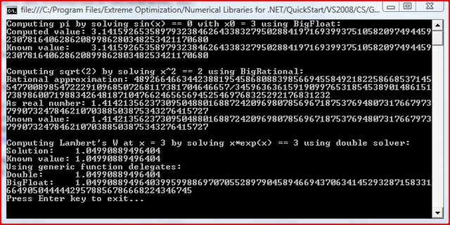
The number PI is often labeled 3.14… and so on. PI, however, is a transcendental number. Computing PI to millions of places will result in a series of places that literally show no pattern. This has often baffled mathematicians. If we use a generic algorithm, we can compute PI to, say, 100 places to verify this. Another example is the square root of 2. It is often labeled 1.414. The inverse of 1.414 is .707, which in referred to the “average peak current” in basic electrical engineering. These and other examples are often best solved by using the computational models of a generic algorithm. Here is an example:

using System;
using Extreme.Mathematics.Generic;
using Extreme.Mathematics;
public class GenericAlgorithms
 {
   public static void Main(string[] args)
    {
           
    Console.WriteLine("Computing pi by solving sin(x) == 0 with x0 = 3 using BigFloat:");
           
       Solver<bigfloat> bigFloatSolver = new Solver<bigfloat>();
       // Set the function to solve, and its derivative.
       bigFloatSolver.TargetFunction = 
       delegate(BigFloat x) { return BigFloat.Sin(x); };
       bigFloatSolver.DerivativeOfTargetFunction = 
       delegate(BigFloat x) { return BigFloat.Cos(x); };
       // Now solve to within a tolerance of 10^-100.
       BigFloat pi = bigFloatSolver.Solve(3, BigFloat.Pow(10, -100));
       // Print the results...
       Console.WriteLine("Computed value: {0:F100}", pi);
       // and verify:
       Console.WriteLine("Known value:    {0:F100}", 
       BigFloat.GetPi(AccuracyGoal.Absolute(100)));
       Console.WriteLine();

       // Next, we will use rational numbers to compute
       // an approximation to the square root of 2.
       Console.WriteLine("Computing sqrt(2) by solving x^2 == 2 using BigRational:");
       // Create the solver...
       Solver<bigrational> bigRationalSolver = new Solver<bigrational>();
       // Set properties...
       bigRationalSolver.TargetFunction = 
       delegate(BigRational x) { return x * x - 2; };
       bigRationalSolver.DerivativeOfTargetFunction =
       delegate(BigRational x) { return 2 * x; };
       // Compute the solution...
       BigRational sqrt2 = bigRationalSolver.Solve(1, BigRational.Pow(10, -100));
       // And print the result.
       Console.WriteLine("Rational approximation: {0}", sqrt2);
       // To verify, we convert the BigRational to a BigFloat:
       Console.WriteLine("As real number: {0:F100}", 
       new BigFloat(sqrt2, AccuracyGoal.Absolute(100), RoundingMode.TowardsNearest));
       Console.WriteLine("Known value:    {0:F100}", 
       BigFloat.Sqrt(2, AccuracyGoal.Absolute(100), RoundingMode.TowardsNearest));
       Console.WriteLine();

       // Now, we compute the Lambert W function at x = 3.
       Console.WriteLine("Computing Lambert's W at x = 3
       by solving x*exp(x) == 3 using double solver:");
       // Create the solver...
       Solver<double> doubleSolver = new Solver<double>();
       // Set properties...
       doubleSolver.TargetFunction = delegate(double x) { return x * Math.Exp(x) - 3; };
       doubleSolver.DerivativeOfTargetFunction = 
       delegate(double x) { return Math.Exp(x) * (1 + x); };
       // Compute the solution...
       double W3 = doubleSolver.Solve(1.0, 1e-15);
       // And print the result.
       Console.WriteLine("Solution:    {0}", W3);
       Console.WriteLine("Known value: {0}", 
       Extreme.Mathematics.ElementaryFunctions.LambertW(3.0));

       // Finally, we use generic functions:
       Console.WriteLine("Using generic function delegates:");
      // The delegates are slightly more complicated.
       doubleSolver.TargetFunction = fGeneric<double>;
       doubleSolver.DerivativeOfTargetFunction = dfGeneric<double>;
       double genericW3 = doubleSolver.Solve(1, 1e-15);
       Console.WriteLine("Double:      {0}", genericW3);
       bigFloatSolver.TargetFunction = fGeneric<bigfloat>;
       bigFloatSolver.DerivativeOfTargetFunction = dfGeneric<bigfloat>;
       BigFloat bigW3 = bigFloatSolver.Solve(1, BigFloat.Pow(10, -100));
       Console.WriteLine("BigFloat:    {0:F100}", bigW3);

      Console.Write("Press Enter key to exit...");
      Console.ReadLine();
        }

      // Generic versions of the above
      static T fGeneric<t><T>(T x)
        {
          IRealOperations<t><T> ops =
          (IRealOperations<t><T>)TypeAssociationRegistry.GetInstance(
                    typeof(T), TypeAssociationRegistry.ArithmeticKey);
            return ops.Subtract(
                ops.Multiply(x, ops.Exp(x)),
                ops.FromInt32(3));
        }
        static T dfGeneric<t><T>(T x)
        {
            IRealOperations<t><T> ops =
                (IRealOperations<t><T>)TypeAssociationRegistry.GetInstance(
                    typeof(T), TypeAssociationRegistry.ArithmeticKey);
            return ops.Multiply(
                ops.Exp(x),
                ops.Add(x, ops.One));
        }
    }

    /// <summary>
    /// Class that contains the generic Newton-Raphson algorithm.
    /// </summary>
    /// <typeparam name="T">The operand type.</typeparam>
    class Solver<T><t>
    {
        // Use a static variable to hold the arithmetic instance.
        // We get the instance from the global TypeAssociationRegistry:
        static IFieldOperations<t><T> ops = 
            (IFieldOperations<t><T>)TypeAssociationRegistry.GetInstance(
                typeof(T), TypeAssociationRegistry.ArithmeticKey);

        // Member fields:
        GenericFunction<t><T> f, df;
        int maxIterations = 100;

        // The function to solve:
        public GenericFunction<t><T> TargetFunction
        {
            get { return f; }
            set { f = value; }
        }
        // The derivative of the function to solve.
        public GenericFunction<t><T> DerivativeOfTargetFunction
        {
            get { return df; }
            set { df = value; }
        }
        // The maximum number of iterations.
        public int MaxIterations
        {
            get { return maxIterations; }
            set { maxIterations = value; }
        }

        // The core algorithm.
        // Arithmetic operations are replaced by calls to
        // methods on the arithmetic object (ops).
        public T Solve(T initialGuess, T tolerance)
        {
            int iterations = 0;

            T x = initialGuess;
            T dx = ops.Zero;
            do
            {
                iterations++;
                // Compute the denominator of the correction term.
                T dfx = df(x);
                // Relational operators map to the Compare method.
                // We also use the value of zero for the operand type.
                // if (dfx == 0)
                if (ops.Compare(dfx, ops.Zero) == 0)
                {
                    // Change value by 2x tolerance.
                    // When multiplying by a power of two, it's more efficient 
                    // to use the ScaleByPowerOfTwo method.
                    dx = ops.ScaleByPowerOfTwo(tolerance, 1);
                }
                else
                {
                    // dx = f(x) / df(x)
                    dx = ops.Divide(f(x), dfx);
                }
                // x -= dx;
                x = ops.Subtract(x, dx);
                                
                // if |dx|^2<tolerance>< 0)
                    return x;
            }
            while (iterations < MaxIterations);
            return x;
        }
    }

By the way, this is a prime example of how well Visual Studio and the .NET Framework can both interoperate and integrate other components to achieved a desired result. Most people who start out learning managed code feel that there could be limitations, but there are not. Integrating the Numerical Library for .NET enables us to write an algorithm in managed code. Here is the output:

For the sake of extending the System.Math APIs defined in the BCL, consider this code:

using System; 
 public class Application
  {
   public static void Main()
    {
      Console.WriteLine("Abs({0}) = {1}", -55, Math.Abs(-55));
      Console.WriteLine("Ceiling({0}) = {1}", 55.3, Math.Ceiling(55.3));
      Console.WriteLine("Pow({0},{1}) = {2}", 10.5, 3, Math.Pow(10.5, 3));
      Console.WriteLine("Round({0},{1}) = {2}",
                10.55358, 2, Math.Round(10.55358, 2));
      Console.WriteLine("Sin({0}) = {1}", 323.333, Math.Sin(323.333));
      Console.WriteLine("Cos({0}) = {1}", 323.333, Math.Cos(323.333));
      Console.WriteLine("Tan({0}) = {1}", 323.333, Math.Tan(323.333));
     }
   }

Simple enough? We just plug in some values to math functions and get the result:

Abs(-55) = 55
Ceiling(55.3) = 56
Pow(10.5,3) = 1157.625
Round(10.55358,2) = 10.55
Sin(323.333) = 0.248414709883854
Cos(323.333) = -0.968653772982546
Tan(323.333) = -0.256453561440193

Outputting results can help in very basic computations for those who work with math, either professionally or educationally. But when we can construct polynomials, complex numbers, perform extended calculations with managed code, we have neared languages like FORTRAN, Ada, LISP, and other scientific computing languages. Now while our focus has been on C#, we will take a look at polynomials using the F# interactive. So we launch the interactive, set the path to where the DLLs reside, reference the Extreme.Numerics.Net20.dll, and then open up the reference to the .NET Framework’s System namespace. Here is a view:

Here is the remainder of the code:

open System
 
// The Polynomial class resides in the Extreme.Mathematics.Curves namespace.
open Extreme.Mathematics.Curves
 
// 1st option: a polynomial of a specified degree.
let polynomial1 = new Polynomial(3)
// Now set the coefficients individually. The coefficients
// can be set using the indexer property. The constant term 
// has index 0:
 
polynomial1.Coefficient(3) <- 1.0
polynomial1.Coefficient(2) <- 1.0
polynomial1.Coefficient(1) <- 0.0
polynomial1.Coefficient(0) <- -2.0
 
// 2nd option: specify the coefficients in the constructor
// as an array of doubles:
let coefficients = [| -2.0; 0.0; 1.0; 1.0 |]
let polynomial2 = new Polynomial(coefficients)
 
// In addition; you can create a polynomial that
// has certain roots using the static FromRoots
// method:
let roots = [| 1.0; 2.0; 3.0; 4.0 |]
let polynomial3 = Polynomial.FromRoots(roots)
// Or you can construct the interpolating polynomial
// by calling the static GetInterpolatingPolynomial
// method. The parameters are two double arrays 
// containing the x values and y values respectively.
let xValues = [| 1.0; 2.0; 3.0; 4.0 |]
let yValues = [| 1.0; 4.0; 10.0; 8.0 |]
let polynomial4 = Polynomial.GetInterpolatingPolynomial(xValues, yValues)
 
// The ToString method gives a common string
// representation of the polynomial:
Console.WriteLine("polynomial3 = {0}", polynomial3.ToString())
 
//
// Curve Parameters
//
 
// The shape of any curve is determined by a set of parameters.
// These parameters can be retrieved and set through the
// Parameters collection. The number of parameters for a curve 
// is given by this collection's Count property.
//
// For polynomials, the parameters are the coefficients
// of the polynomial. The constant term has index 0:
Console.WriteLine("polynomial1.Parameters.Count = {0}", polynomial1.Parameters.Count)
// Parameters can easily be retrieved:            
Console.Write("polynomial1 parameters:")
for index = 0 to polynomial1.Parameters.Count - 1 do
  Console.Write("{0} ", polynomial1.Parameters.[index])
done
Console.WriteLine()
// We can see that polynomial2 defines the same polynomial 
// curve as polynomial1:
Console.Write("polynomial2 parameters:")
for index = 0 to polynomial2.Parameters.Count - 1 do
  Console.Write("{0} ", polynomial2.Parameters.[index])
done
Console.WriteLine()
// Parameters can also be set:
polynomial2.Parameters.[0] <- 1.0
 
// For polynomials and other classes that inherit from
// the LinearCombination class, the parameters are also
// available through the indexer property of Polynomial.
// The following is equivalent to the line above:
polynomial2.Coefficient(0) <- 1.0
Console.WriteLine(polynomial2.Coefficient(2))
 
// The degree of the polynomial is returned by
// the Degree property:
Console.WriteLine("Degree of polynomial3 = {0}", 
polynomial3.Degree)
 
//
// Curve Methods
//
 
// The ValueAt method returns the y value of the
// curve at the specified x value:
Console.WriteLine("polynomial1.ValueAt(2) = {0}", polynomial1.ValueAt(2.0))
 
// The SlopeAt method returns the slope of the curve
// a the specified x value:
Console.WriteLine("polynomial1.SlopeAt(2) = {0}", polynomial1.SlopeAt(2.0))
 
// You can also create a new curve that is the 
// derivative of the original:
let derivative = polynomial1.GetDerivative()
Console.WriteLine("Slope at 2 (derivative) = {0}", derivative.ValueAt(2.0))
// For a polynomial, the derivative is a Quadratic curve
// if the degree is equal to three:
Console.WriteLine("Type of derivative: {0}", derivative.GetType().FullName)
Console.Write("Derivative parameters: ")
 
for index = 0 to derivative.Parameters.Count - 1 do
  Console.Write("{0} ", derivative.Parameters.[index])
done
Console.WriteLine()
// If the degree is 4 or higher, the derivative is
// once again a polynomial:
Console.WriteLine("Type of derivative for polynomial3: 
 {0}", polynomial3.GetDerivative().GetType().FullName)
 
// You can get a Line that is the tangent to a curve
// at a specified x value using the TangentAt method:
let tangent = polynomial1.TangentAt(2.0)
Console.WriteLine("Tangent line at 2:")
Console.WriteLine("  Y-intercept = {0}", tangent.Parameters.[0])
Console.WriteLine("  Slope = {0}", tangent.Parameters.[1])
 
// For many curves, you can evaluate a definite
// integral exactly:
Console.WriteLine("Integral of polynomial1
 between 0 and 1 = {0}", polynomial1.Integral(0.0, 1.0))
 
// You can find the zeroes or roots of the curve
// by calling the FindRoots method. Note that this
// method only returns the real roots.
roots = polynomial1.FindRoots()
Console.WriteLine("Number of roots of polynomial1: 
{0}", roots.Length)
Console.WriteLine("Value of root 1 = {0}", roots.[0])
// Let's find polynomial3's roots again:
roots = polynomial3.FindRoots()
Console.WriteLine("Number of roots of polynomial3: 
{0}", roots.Length)
Console.WriteLine("Value of root = {0}", roots.[0])
Console.WriteLine("Value of root = {0}", roots.[1])
// Root finding isn't an exact science. Note the 
// round-off error in these values:
Console.WriteLine("Value of root = {0}", roots.[2])
Console.WriteLine("Value of root = {0}", roots.[3])
  
Console.Write("Press Enter key to exit...")
Console.ReadLine()

Here is the output:

If you are familiar with F#, then you will recognize the type inference by pressing the enter key upon completion:

val polynomial1 : Extreme.Mathematics.Curves.Polynomial = x^3+x^2-2
val coefficients : float [] = [|-2.0; 0.0; 1.0; 1.0|]
val polynomial2 : Extreme.Mathematics.Curves.Polynomial = x^3+x^2+1
val roots : float [] = [|1.0; 2.0; 3.0; 4.0|]
val polynomial3 : Extreme.Mathematics.Curves.Polynomial =
  x^4-10x^3+35x^2-50x+24
val xValues : float [] = [|1.0; 2.0; 3.0; 4.0|]
val yValues : float [] = [|1.0; 4.0; 10.0; 8.0|]
val polynomial4 : Extreme.Mathematics.Curves.Polynomial =
  -1.83333333333333x^3+12.5x^2-21.6666666666667x+12
val derivative : Extreme.Mathematics.Curves.Curve = 3x^2+2x
val tangent : Extreme.Mathematics.Curves.Line = 16x-22

One of the most daunting tasks math students and professionals face regularly is writing an equation that will, when values are plugged in, result in a solution (or estimation) of a certain problem that is mathematical.