Introduction
The frequency analysis is the one of the most popular methods in signal processing. It is a tool for signal decomposition for further filtration, which is in fact separation of signal components from each other.
Although, the process of crossing the border between these two worlds (time and frequency domain) may be considered as advanced case, it is worth doing it, as this other world gives us new opportunities and simplifies many issues.
The article presents implementation of the various versions of calculating Discrete Fourier Transform, starting with definition of Fourier Transform, by reduced calculation algorithm and finishing with Cooley-Tukey method of Fast Fourier Transform.
In addition, it presents the importance of the simplest operations performed on the signal spectrum and their impact on the time domain.
Signals
Signal can be defined as a variability of any physical value, that can be described as a function of a single or multiple arguments. In this article we will be interested in one-dimensional time functions.
In real world, time functions that can be met are placed in continuous domain. However, the development of computer science, caused that analog signal processing became rare. It is much more cost-effective to create, implement and test signal processing algorithms in digital world, then to project and develop analog (electronic) devices.
From continuous to discrete domain
In order to receive digital representation of analog signal it needs to be turned into discrete-time domain and quantized.
The Nyquist-Shannon sampling theorem is the link between continuous-time signals and discrete-time signals. This theorem can be also known as The Whittaker-Nyquist-Kotielnikov-Shannon sampling theorem – the choice of the authors names depending on the country in which we talk about this issue. To be above this, we will call it simply the sampling theorem.
The sampling theorem answers the question of how to sample a continuous-time signal to obtain a discrete-time signal, from which you can restore original (continuous-time) signal. According to this statement to obtain a properly sampled discrete-time signal, the sampling frequency must be at least twice of highest frequency that can be observed in original signal.
Signal decomposition into frequency domain
It all started in 1807 when the French mathematician and physicist, Joseph Fourier, introduced the trigonometric series decomposition (nowadays know as Fourier series method) to solve the partial differential heat equation in the metal plate. Fourier's idea was to decomposed complicated periodic function into to sum of the simplest oscillating functions - sines ans cosines.

Joseph Fourier
If the function f(x) is periodic with period of T and intergrable (its integral is finite) on an interval [x0, x0 + T], then it can be transformed into series:
$\begin{aligned} f(x) = \frac{a_0}{2} + \sum_{n=1}^{\infty} (a_n \cdot cos(\frac{2 n \pi}{T}x) + b_n \cdot sin(\frac{2 n \pi}{T}x)) \end{aligned}$
where
$\begin{aligned} a_n = \frac{2}{T} \int_{x_0}^{x_0 + T} f(x) \cdot cos(\frac{2 n \pi}{T}x) dx \\ b_n = \frac{2}{T} \int_{x_0}^{x_0 + T} f(x) \cdot sin(\frac{2 n \pi}{T}x) dx \end{aligned}$
Discrete Fourier Transform
Definition
Fourier series can be named a progenitor of Fourier Transform, which, in case of digital signals (Discrete Fourier Transform), is described with formula:
$\begin{aligned} X(k) = \frac{1}{N} \sum_{n=0}^{N-1} x(n) \cdot e^{-j \frac{2 \pi}{N} k n } \end{aligned}$
Fourier transformation is reversible and we can return to time domain by calculation:
$\begin{aligned} x(n) = \sum_{k=0}^{N-1} X(k) \cdot e^{j \frac{2 \pi}{N} k n } \end{aligned}$
In some notations we can observe that divide by N is transterred to inverse calculation - it does not disrupt the calculation unless we apply divide by N both in forward and inverse Fourier Transform.
Forward and inverse Discrete Fourier Transform implementations are shown below.
public Complex[] DFT(Double[] x)
{
int N = x.Length;
Complex[] X = new Complex[N];
for (int k = 0; k < N; k++)
{
X[k] = 0;
for (int n = 0; n < N; n++)
{
X[k] += x[n] * Complex.Exp(-Complex.ImaginaryOne * 2 * Math.PI * (k * n) / Convert.ToDouble(N));
}
X[k] = X[k] / N;
}
return X;
}
public Double[] iDFT(Complex[] X)
{
int N = X.Length;
Double[] x = new Double[N];
for (int n = 0; n < N; n++)
{
Complex sum = 0;
for (int k = 0; k < N; k++)
{
sum += X[k] * Complex.Exp(Complex.ImaginaryOne * 2 * Math.PI * (k * n) / Convert.ToDouble(N));
}
x[n] = sum.Real;
}
return x;
}
The mistake often committed in code implementation of inverse Fourier Transform is to transfer complex value to real by using its magnitude value - in such a case we will receive |x(n)| instead of x(n).
Practical example of Discrete Fourier Transform calculated by definition
To verify algorithm let us create a signal that is a sum of two sine waves:
$\begin{aligned} x_1(n) = sin(0.02 \pi n) \end{aligned}$
$\begin{aligned} x_2(n) = 0.25 \cdot sin(0.2 \pi n) \end{aligned}$
Denote by x1(n) an original signal and by x2(n) a disruption signal (noise). The sum of those signals x(n) = x1(n)+x2(n) is in that case a disrupted signal.
$\begin{aligned} x(n) = x_1(n) + x_2(n) \end{aligned}$
$\begin{aligned} n = 0, 1, ..., 100 \end{aligned}$


Fig.1. Original and disruption signals
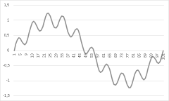
Fig.2. The sum of signals (disrupted signal)
As we created our signal from the sum of two sine waves, then according to the Fourier theorem we should receive its frequency image concentrated around two frequencies f1 and f2 and also its opposites -f1 and -f2.

Fig.3. Amplitude spectrum of disrupted singal.
If Fourier theorem is correct, then by removing from spectrum stripes that came from disruption signal, we should receive original signal.

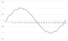
Fig.4. Spectrum with removed disruption frequency and its inverse DFT result
As we can observe in figure 4, our output signal is close to original one and the distortions are caused by additional stripes have arisen as a result of numerical operations. Let's remove them all, and leave only two main stripes.


Fig.5. Spectrum with only main frequency and its inverse DFT result.
The output signal in figure 5 looks like perfect sine wave. But to show minor differences between output and original signal see comparison below.

Fig.6. Original and output signal comparison.
In figure 3 we cannot see any negative values, so why did we said, that calculated spectrum is concentrated around two frequencies f1 and f2 and also its opposites -f1 and -f2?
It is because we get use to analyze signals which are defined in range symmetric to the origin. If we denote our disrupted signal x(n) as:
$\begin{aligned} x(n) = x_1(n) + x_2(n) \end{aligned}$
$\begin{aligned} n = -50, -49, ..., -1, 0, 1, ..., 49, 50 \end{aligned}$
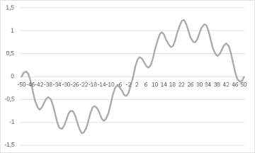
Fig.7. Shifted signal
and implement minor change in our algorithm:
public Complex[] DFT(Double[] x, int[] SamplesNumbers)
{
int N = x.Length;
Complex[] X = new Complex[N];
for (int k = 0; k < N; k++)
{
X[k] = 0;
Double s1 = SamplesNumbers[k];
for (int n = 0; n < N; n++)
{
Double s2 = SamplesNumbers[n];
X[k] += x[n] * Complex.Exp(-Complex.ImaginaryOne * 2 * Math.PI * (s1 * s2) / Convert.ToDouble(N));
}
X[k] = X[k] / N;
}
return X;
}
we will receive amplitude spectrum shown below.

Fig.8. Amplitude spectrum of shifted signal
The same change needs to be implemented in inverse DFT method.
public Double[] iDFT(Complex[] X, int[] SamplesNumbers)
{
int N = X.Length;
Double[] x = new Double[N];
for (int n = 0; n < N; n++)
{
Complex sum = 0;
Double s1 = SamplesNumbers[n];
for (int k = 0; k < N; k++)
{
Double s2 = SamplesNumbers[k];
sum += X[k] * Complex.Exp(Complex.ImaginaryOne * 2 * Math.PI * (s1 * s2) / Convert.ToDouble(N));
}
x[n] = sum.Real;
}
return x;
}
Notice, that by shifting signal to symmetrical position to the orgin, we calculated shifted spectrum:
$\begin{aligned} X(k) \rightarrow X(k - \frac{N}{2}) \end{aligned}$
The same effect can be achieved, if we change original signal using formula
$\begin{aligned} x(n) \rightarrow (-1)^n \cdot x(n) \end{aligned}$
In this case, there is no need to store the actual numbers of samples. For this use the method is shown below.
public Double[] Shift(Double[] x)
{
int N = x.Length;
for (int i = 0; i < N; i++)
{
x[i] = (int)Math.Pow(-1, i) * x[i];
}
return x;
}
Discrete Fourier Transform with a reduced number of calculations
Let us look again at the forward Discrete Fourier Transform definition:
$\begin{aligned} X(k) = \frac{1}{N} \sum_{n=0}^{N-1} x(n) \cdot e^{-j \frac{2 \pi}{N} k n } \end{aligned}$
Denote by WN auxiliary variable:
$\begin{aligned} W_N = e^{-j \frac{2 \pi }{N}}\end{aligned}$
Then our formula takes the form
$\begin{aligned} X(k) = \frac{1}{N} \sum_{n=0}^{N-1} x(n) \cdot W_N ^{k n} \end{aligned}$
Also we can notice that if k = 0 or n = 0 we receive:
$\begin{aligned} W_N^{k n} = 1 \end{aligned}$
Accordingly, the designation of DTF can be written in matrix form:
$\begin{aligned} \begin{bmatrix} X[0] \\ X[1] \\ \vdots \\ X[N-1] \end{bmatrix} = \frac{1}{N} \begin{bmatrix} 1 & 1 & 1 & \dots & 1 \\ 1 & W_N & W_N^2 & \dots & W_N^{N-1} \\ 1 & W_N^2 & W_N^4 & \dots & W_N^{N-2} \\ 1 & W_N^3 & W_N^6 & \dots & W_N^{N-3} \\ \vdots & \vdots & \vdots & \ddots & \vdots \\ 1 & W_N^{N-1} & W_N^{N-2} & \dots & W_N \end{bmatrix} \cdot \begin{bmatrix} x[0] \\ x[1] \\ \vdots \\ x[N-1] \end{bmatrix} \end{aligned}$
It follows that, to determine the Dicrete Fourier Transform of N-samples signal, we have to perform N2 multiplication operations and determine the (N-1)2 coefficients in matrix WN. Remind that multiplication opertion is one of the most time-consuming opertion for processors.
Let us return to factor WN and consider N=4 samples signal x(n). To calculate X(k) we need to find values of matrix coefficients:
$\begin{aligned} \begin{bmatrix} 1 & 1 & 1 & 1 \\ 1 & W_4 & W_4^2 & W_4^3 \\ 1 & W_4^2 & W_4^4 & W_4^2 \\ 1 & W_4^3 & W_4^2 & W_4 \end{bmatrix} \end{aligned}$
We have:
$\begin{aligned} W_4 = e^{-j \frac{\pi}{2}} = cos(-\frac{\pi}{2}) + j \cdot sin(-\frac{\pi}{2}) = cos(\frac{\pi}{2}) - j \cdot sin(\frac{\pi}{2}) = -j \end{aligned}$
where
$\begin{aligned} e^{j \phi} = cos(\phi) + j \cdot sin(\phi) \end{aligned}$
is the Euler's formula.
Next values are
$\begin{aligned} \begin{matrix} W_4^2 = -1 \\ W_4^3 = j \\ W_4^4 = -1 \end{matrix} \end{aligned}$
Notice that
$\begin{aligned} \begin{matrix} W_4^2 = -W_4^0 \\ W_4^3 = -W_4^1 \end{matrix} \end{aligned}$
Similar situation can be noticed for N=8:
$\begin{aligned} \begin{matrix} W_8^1 = e^{-j \frac{\pi}{4}} = cos(\frac{\pi}{4}) - j \cdot sin(\frac{\pi}{4}) = \frac{\sqrt{2}}{2}(1 - j) = \frac{1-j}{\sqrt{2}} \\ W_8^2 = (\frac{(1-j)^2}{2}) = -j \\ W_8^3 = -j \cdot \frac{1-j}{\sqrt{2}} = \frac{-1-j}{\sqrt{2}} \\ W_8^4 = \frac{-1-j}{\sqrt{2}} \cdot \frac{1-j}{\sqrt{2}} = -1 \\ W_8^5 = - \frac{1-j}{\sqrt{2}} \\ W_8^6 = - (\frac{1-j}{\sqrt{2}})^2 = j \\ W_8^7 = j \cdot \frac{1-j}{\sqrt{2}} = \frac{1+j}{\sqrt{2}} \\ W_8^8 = \frac{1+j}{\sqrt{2}} \cdot \frac{1-j}{\sqrt{2}} = 1 \end{matrix} \end{aligned}$
that provides to:
$\begin{aligned} \begin{matrix} W_8^4 = -W_8^0 \\ W_8^5 = -W_8^1 \\ W_8^6 = -W_8^2 \\ W_8^7 = -W_8^3 \end{matrix} \end{aligned}$
In general, for N-samples signal we can write:
$\begin{aligned} \begin{matrix} W_N^z = - W_N^{z - \frac{N}{2}} \\ z = \frac{N}{2}, \frac{N}{2} + 1, \frac{N}{2} + 2, ..., N \end{matrix}\end{aligned}$
This observation leads us to the conclusion that in determining the DFT we calculate only N/2 - 1 spectral coefficients, and another we can get from the previous ones - it is a property of symmetry of the spectrum. Due to this observation four times reduced the number of operations within the algorithm. This observation is true only if we deal with the physical signals, that is signals with real values.
public Complex[] DFT2(Double[] x)
{
int N = x.Length;
Complex[] X = new Complex[N];
X[0] = x.Sum() / N;
for (int k = 1; k < N/2 + 1; k++)
{
X[k] = 0;
for (int n = 0; n < N; n++)
{
X[k] += x[n] * Complex.Exp(-Complex.ImaginaryOne * 2 * Math.PI * (k * n) / Convert.ToDouble(N));
}
X[k] = X[k] / N;
if (k != N / 2)
{
X[N - k] = new Complex(X[k].Real, -X[k].Imaginary);
}
}
return X;
}
public Complex[] DFT2(Double[] x, int[] SamplesNumbers)
{
int N = x.Length;
Complex[] X = new Complex[N];
for (int k = 0; k < N / 2 + 1; k++)
{
X[k] = 0;
Double s1 = SamplesNumbers[k];
for (int n = 0; n < N; n++)
{
Double s2 = SamplesNumbers[n];
X[k] += x[n] * Complex.Exp(-Complex.ImaginaryOne * 2 * Math.PI * (s1 * s2) / Convert.ToDouble(N));
}
X[k] = X[k] / N;
if (k != N/2)
{
X[N - k - 1] = new Complex(X[k].Real, -X[k].Imaginary);
}
}
return X;
}
Examples:

Fig.9. Amplitude spectrum of signal from fig.2. designated with DFT with reduced number of calculation

Fig.10. Amplitude spectrum of signal from fig.7. designated with DFT with reduced number of calculation
Fast Fourier Transform
Fourier Transform formula can be splitted into:
$\begin{aligned} X(k) = \frac{1}{N} \sum_{n=0}^{N-1} x(n) \cdot e^{-j \frac{2 \pi}{N} k n } = \frac{1}{N} \sum_{n=0}^{\frac{N}{2}-1} x(2n) \cdot W_N^{2nk} + \frac{1}{N} \sum_{n=0}^{\frac{N}{2}-1} x(2n + 1) \cdot W_N^{(2n+1)k} \end{aligned}$
where
$\begin{aligned} W_N^{2nk} = e^{-j \frac{2 \pi}{N} 2 n k} = e^{-j \frac{2 \pi}{\frac{N}{2}}nk} = W_{\frac{N}{2}}^{n k} \end{aligned}$
and
$\begin{aligned} W_N^{(2n+1)k} = W_N^{2nk + k} = W_N^{2nk} \cdot W_N^{k} = W_{\frac{N}{2}}^{n k} \cdot W_N^{k} \end{aligned}$
therefore:
$\begin{aligned} X(k) = \frac{1}{N} \sum_{n=0}^{\frac{N}{2}-1} x(2n) \cdot W_{\frac{N}{2}}^{n k} + \frac{1}{N} \cdot W_N^{k} \sum_{n=0}^{\frac{N}{2}-1} x(2n + 1) \cdot W_{\frac{N}{2}}^{n k} \end{aligned}$
that can be written in a simpler form, that separates the calculations performed for the even samples, from those performed for the odd ones:
$\begin{aligned} X(k) = X_E(k) + W_N^k \cdot X_O(k) \end{aligned}$
Accordingly, referring to our previous calculations for the case N = 8 can be written as:
$\begin{aligned} \begin{matrix} X(0) = X_E(0) + W_8^0 \cdot X_O(0) \\ X(1) = X_E(1) + W_8^1 \cdot X_O(1) \\ X(2) = X_E(2) + W_8^2 \cdot X_O(2) \\ X(3) = X_E(3) + W_8^3 \cdot X_O(3) \\ X(4) = X_E(0) + W_8^4 \cdot X_O(0) = X_E(0) - W_8^0 \cdot X_O(0) \\ X(5) = X_E(1) + W_8^5 \cdot X_O(1) = X_E(1) - W_8^1 \cdot X_O(1) \\ X(6) = X_E(2) + W_8^6 \cdot X_O(2) = X_E(2) - W_8^2 \cdot X_O(2) \\ X(7) = X_E(3) + W_8^7 \cdot X_O(3) = X_E(3) - W_8^3 \cdot X_O(3) \\ \end{matrix} \end{aligned}$
which can be presented as graph:
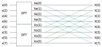
Fig.11. DFT decomposition into even and odd samples calculation.
Note that the elements:
 and
and 
can be calculated in the same way: elements x(0), x(4), x(1) and x(5) are in their diagrams the even indices, whereas x(2), x(6), x(3) and x(7) are the odd ones. Combining them in the ordered pairs, the above graphs can be redraw:

Finally, in this example:

Fig.12. Fast Fourier Transform (RADIX-2) for N = 8 signal.
Designating DFT definition for N = 8 signal we had to perform 64 operations of multiplication, but due to the above observation, we made them only 12. The greater the number of samples in the signal, the greater benefit in calculations number with the use of the FFT algorithm, since the amount of calculations for N-smaple signal can be determined as:
$\begin{aligned} \begin{matrix} \frac{N}{2} log_2(N) \end{matrix} \end{aligned}$
The basic element of such a calculation is called "butterfly":

where
$\begin{aligned} \begin{matrix} Y(k) = y(k) + W_N^k \cdot y(k + \frac{N}{2}) \\ Y(k + \frac{N}{2}) = y(k) - W_N^k \cdot y(k + \frac{N}{2}) \end{matrix} \end{aligned}$
Successive decomposition stages for smaller, down to the basic "butterflies" may be carried out only on the assumption that N is a power of 2.
Fast Fourier Transform in practice
Proper number of samples
The easiest way to processed signal have the number of samples which is a power of 2, simply fill in the missing samples of zeros. Depending on the signal structure, additions can be made as right-hand, left-hand or both sides.

Fig.13. Complemented signal from fig.2
Sorting samples
To connect consecutive signal samples in the respective pairs, we are using preliminary sorting algorithms. However, the FFT algorithm can be performed on samples unsorted, and the sorting operation (in the same way) can be performed on the samples of the spectrum.
In the hardware spectrum analyzers and low-level programming languages sorting samples it is much easier, because the operation is based on a simple inversion of bits in the binary representation of the index sample.
In our N = 8 signal we can notice that:
$\begin{aligned} \begin{matrix} x(0) & 000 & \rightarrow & 000 & x(0) \\ x(1) & 001 & \rightarrow & 100 & x(4) \\ x(2) & 010 & \rightarrow & 010 & x(2) \\ x(3) & 011 & \rightarrow & 110 & x(6) \\ x(4) & 100 & \rightarrow & 001 & x(1) \\ x(5) & 101 & \rightarrow & 101 & x(5) \\ x(6) & 110 & \rightarrow & 011 & x(3) \\ x(7) & 111 & \rightarrow & 111 & x(7) \end{matrix} \end{aligned}$
Method implementation in general case:
public Double[] FFTDataSort(Double[] x)
{
int N = x.Length;
if (Math.Log(N, 2) % 1 != 0)
{
throw new Exception("Number of samples in signal must be power of 2");
}
Double[] y = new Double[N];
int BitsCount = (int)Math.Log(N, 2);
for (int n = 0; n < N; n++)
{
string bin = Convert.ToString(n, 2).PadLeft(BitsCount, '0');
StringBuilder reflection = new StringBuilder(new string('0', bin.Length));
for (int i = 0; i < bin.Length; i++)
{
reflection[bin.Length - i - 1] = bin[i];
}
int number = Convert.ToInt32(reflection.ToString(),2);
y[number] = x[n];
}
return y;
}
This operation can, however, be performed much faster, without need to convert the index number to the binary form:
public Double[] FFTDataSort2(Double[] x)
{
int N = x.Length;
if (Math.Log(N, 2) % 1 != 0)
{
throw new Exception("Number of samples in signal must be power of 2");
}
int m = 1;
for (int n = 0; n < N - 1; n++)
{
if (n < m)
{
Double T = x[m-1];
x[m-1] = x[n];
x[n] = T;
}
int s = N / 2;
while (s < m)
{
m = m - s;
s = s / 2;
}
m = m + s;
}
return x;
}
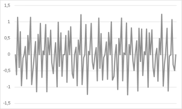
Fig.14. Sorted signal samples (signal from fig.2. complemented at the right side)
Fast Fourier Transfom algorithm
FFT algorithm implementation is shown below.
public Complex[] FFT(Double[] x)
{
int N = x.Length;
if (Math.Log(N, 2) % 1 != 0)
{
throw new Exception("Number of samples in signal must be power of 2");
}
Complex[] X = new Complex[N];
for (int i = 0; i < N; i++)
{
X[i] = new Complex(x[i], 0);
}
int S = (int)Math.Log(N, 2);
for (int s = 1; s < S + 1; s++)
{
int BW = (int)Math.Pow(2, s - 1);
int Blocks = (int)(Convert.ToDouble(N) / Math.Pow(2, s));
int BFlyBlocks = (int)Math.Pow(2, s - 1);
int BlocksDist = (int)Math.Pow(2, s);
Complex W = Complex.Exp(-Complex.ImaginaryOne * 2 * Math.PI / Math.Pow(2, s));
for (int b = 1; b < Blocks + 1; b++)
{
for (int m = 1; m < BFlyBlocks + 1; m++)
{
int itop = (b - 1) * BlocksDist + m;
int ibottom = itop + BW;
Complex Xtop = X[itop-1];
Complex Xbottom = X[ibottom-1] * Complex.Pow(W, m - 1);
X[itop-1] = Xtop + Xbottom;
X[ibottom-1] = Xtop - Xbottom;
}
}
}
for (int i = 0; i < N; i++)
{
X[i] = X[i] / Convert.ToDouble(N);
}
return X;
}
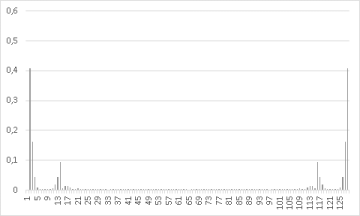
Fig.15. FFT - Amplitude spectrum of signal with sorted samples (from fig.14)

Fig.16. FFT - Amplitude spectrum of shifted signal with sorted samples (from fig.14)
Inverse Fast Fourier Transform can be implemented by minor change in forward FFT method:
public Double[] iFFT(Complex[] X)
{
int N = X.Length;
Double[] x = new Double[N];
int E = (int)Math.Log(N, 2);
for (int e = 1; e < E + 1; e++)
{
int SM = (int)Math.Pow(2, e - 1);
int LB = (int)(Convert.ToDouble(N) / Math.Pow(2, e));
int LMB = (int)Math.Pow(2, e - 1);
int OMB = (int)Math.Pow(2, e);
Complex W = Complex.Exp(Complex.ImaginaryOne * 2 * Math.PI / Math.Pow(2, e));
for (int b = 1; b < LB + 1; b++)
{
for (int m = 1; m < LMB + 1; m++)
{
int g = (b - 1) * OMB + m;
int d = g + SM;
Complex xgora = X[g - 1];
Complex xdol = X[d - 1] * Complex.Pow(W, m - 1);
X[g - 1] = xgora + xdol;
X[d - 1] = xgora - xdol;
}
}
}
for (int i = 0; i < N; i++)
{
x[i] = X[i].Real;
}
return x;
}

Fig.17. Signal restored from spectrum from fig.15 using inverse Fast Fourier Transform.
As it can be noticed, the signal complemented with additional zero samples is not without effect on the spectrum - at figures 15 and 16 additional stripes can be noticed. Nevertheless, while we keep them for futher calculations, we are able to restore the original signal.
However, let us see if we can still separate the signal from noise and restore it using FFT methods.
Firstly, remove stripes that are suspected of being a disturbance:

Fig.18. Filtred signal spectrum
Secondly, calculate inverse FFT

Fig.19. Inverse FFT - restored signal
Thirdly, cut additional samples

Fig.20. Signal without additional samples.
At the end, compare original (undisturbed) signal with our filtration result.

Fig.21. Original and output signal comparison (Fast Fourier Transform).
Using the code
All signal processing algorithms presented in this article are implemented in attached source code. To start working with DiscreteFourierTransform library simply declare its namespace:
using DiscreteFourierTransform;
create new object:
DiscreteFourierTransform.DiscreteFourierTransform dft = new DiscreteFourierTransform.DiscreteFourierTransform();
and start your adventure with digital signal processing in frequency domain.
Library methods and applications
Test signal
Disturbed sine signal and samples indexes are included in dll:
Double[] signal = dft.testsignal();
int[] n = dft.testsignalindexes();
Discrete Fourier Transform
Complex[] X = dft.DFT(signal);
Double[] A = dft.Amplitude(X);
Complex[] Xa = dft.DFT(signal, n);
Double[] signal2 = dft.Shift(signal);
Complex[] Xb = dft.DFT(signal2);
Inverse Discrete Fourier Transform
Double[] x = dft.iDFT(X);
Double[] xa = dft.iDFT(Xa, n);
Double[] xb = dft.iDFT(Xb);
Discrete Fourier Transform with reduced number of calculation
Complex[] X2 = dft.DFT2(signal);
Complex[] X2a = dft.DFT2(signal, n);
Complex[] X2b = dft.DFT2(dft.Shift(signal), n);
Fast Fourier Transform
Signal pack with zeros
Double[] signalpack = dft.SignalPackRight(signal);
Double[] signalpack2 = dft.SignalPackLeft(signal);
Double[] signalpack3 = dft.SignalPackBoth(signal);
Samples sorting
Double[] signal3 = dft.FFTDataSort(signalpack);
Double[] signal4 = dft.FFTDataSort2(signalpack);
Fast Fourier Transform
Complex[] X3 = dft.FFT(signal3);
Complex[] X3a = dft.FFT(dft.Shift(signal3));
Inverse Fast Fourier Transform
Spectrum stripes sorting
Complex[] X3s = dft.FFTDataSort(X3);
Complex[] X3as = dft.FFTDataSort2(X3);
Inverse Fast Fourier Transform
Double[] x3 = dft.iFFT(X3s);
After graduating with a degree of Master of Science, Engineer in Automation and Robotics (at the Gdansk University of Technology) began his career as a Service Engineer of Ships' Systems. He spent four years in this profession and had a lot of places all over the world visited.
In 2012 he started to work for Polish energy company ENERGA (ENERGA Agregator LLC, ENERGA Innowacje LLC and Enspirion LLC) as Systems Engineer and Solutions Architect. Thereafter he participated in few large-scale research projects in the field of Information Technology and Systems Integration for Energy & Power Management and Demand Response applications as a Solution Architect, Business Architect or Project Manager.
His private interests include Signal and Image Processing, Adaptive Algorithms and Theory of Probability.


 General
  News
News  Suggestion
  Question
  Bug
Bug  Answer
  Joke
Joke  Praise
  Rant
Rant  Admin
Admin 


