Introduction
In this article, we will cover TensorFlow touching the basics and then move to advanced topics. Our focus would be what we can do with TensorFlow.
Background
We won't be defining what exactly Tensorflow is because already there is a lot of content but we will work towards directly using it.
Let's get started.
We are using Anaconda distribution for Python and then install TensorFlow with it. We are working with the GPU version.
We activate the anaconda environment.
We are using Intel optimized python for writing codes in python.
Let's check on how the version on Tensorflow can be seen.

To check the version first, we imported tensorflow.
>>> import tensorflow as tf
>>> print(tf.__version__)
1.1.0

//
Let’s just break the word tensor it means n-dimensional array.
We will create the most basic thing in tensorflow that is constant. We will create a variable named “hello Intel”.
  >>> import tensorflow as tf
>>> hello = tf.constant("Hello ")
>>> Intel = tf.constant("Intel ")
>>> type(Intel)
<class>
>>> print(Intel)
Tensor("Const_1:0", shape=(), dtype=string)
>>> with tf.Session() as sess:
...      result=sess.run(hello+Intel)
Now we print the result.
>>> print(result)
b'Hello Intel '
>>>

</class>
The output in Anaconda prompt window looks like this:
Now let’s work with adding two numbers in TensorFlow.
We declare two variables:
>>> a =tf.constant(50)
>>> b =tf.constant(70)
We again check the type of one of the variables:
>>> type(a)
<class>
</class>
We see the object is of type tensor. For adding two variables, we have to create a session.
>>> with tf.Session() as sess:
...     result = sess.run(a+b)
If we now want to see the result:
>>> result
120
Neural Network from Scratch using TensorFlow
In the next section, we will work around on creating a neural network from scratch in TensorFlow.
In this section, we will create a neural network that performs a simple linear fit to some 2D data.
The steps we will be performing are shown in the figure below.
The structure of the graph for the neural network we are going to construct is shown below.
First of all, we will import numpy and tensorflow.
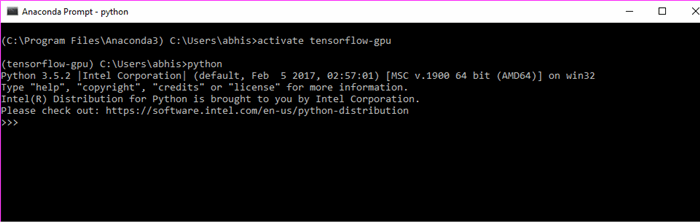
(C:\Program Files\Anaconda3) C:\Users\abhis>activate tensorflow-gpu

(tensorflow-gpu) C:\Users\abhis>python
Python 3.5.2 |Intel Corporation| (default, Feb  5 2017, 02:57:01) [MSC v.1900 64 bit (AMD64)] on win32
Type "help", "copyright", "credits" or "license" for more information.
Intel(R) Distribution for Python is brought to you by Intel Corporation.
Please check out: https://software.intel.com/en-us/python-distribution
>>> import numpy as np
>>> import tensorflow as tf
>>>
We need to set some random seed values for our process.
>>> np.random.seed(101)
>>> tf.set_random_seed(101)
Now, we will add some random data. Using rand_a =np.random.uniform(0,100(5,5)), we add random data points going from 0 to 100 and then ask it to be in the shape of (5,5). We do the same for b.
>>> rand_a =np.random.uniform(0,100,(5,5))
>>> rand_a
array([[ 51.63986277,  57.06675869,   2.84742265,  17.15216562,
         68.52769817],
       [ 83.38968626,  30.69662197,  89.36130797,  72.15438618,
         18.99389542],
       [ 55.42275911,  35.2131954 ,  18.18924027,  78.56017619,
         96.54832224],
       [ 23.23536618,   8.35614337,  60.35484223,  72.89927573,
         27.62388285],
       [ 68.53063288,  51.78674742,   4.84845374,  13.78692376,
         18.69674261]])

>>> rand_b
array([[ 99.43179012],
       [ 52.06653967],
       [ 57.87895355],
       [ 73.48190583],
       [ 54.19617722]])
Now we need to create placeholders for these uniform objects.
>>> a = tf.placeholder(tf.float32)
>>> b = tf.placeholder(tf.float32)
Tensorflow understands normal python operation. We will use it.
>>> add_op = a + b
>>> mul_op = a * b
Now we will create some sessions that use graphs to feed dictionaries to get results. First, we declare the session, then we want to get the results of the add operation. We need to pass in the operation and the feed dictionary. For the placeholder objects, we need to feed data. We will do that by feed dictionary. First, we have the keys, they are a and b, then we pass data to it. add_result = sess.run(add_op,feed_dict={a:10,b:20})
>>> with tf.Session() as sess:
...      add_result = sess.run(add_op,feed_dict={a:10,b:20})
...      print(add_result)
As we have created random, we will pass it to feed dictionary.
>>> with tf.Session() as sess:
...      add_result = sess.run(add_op,feed_dict={a:rand_a,b:rand_b})
Now when we print the value of add_result:
>>> print(add_result)
[[ 151.07165527  156.49855042  102.27921295  116.58396149  167.95948792]
 [ 135.45622253   82.76316071  141.42784119  124.22093201   71.06043243]
 [ 113.30171204   93.09214783   76.06819153  136.43911743  154.42727661]
 [  96.7172699    81.83804321  133.83674622  146.38117981  101.10578918]
 [ 122.72680664  105.98292542   59.04463196   67.98310089   72.89292145]]
We did a matrix addition over here.
We do the same for multiplication too.
>>> with tf.Session() as sess:
...      mul_result = sess.run(mul_op,feed_dict={a:10,b:20})
print(mul_result)
200
Using the random values:
>>> with tf.Session() as sess:
...      mul_result = sess.run(mul_op,feed_dict={a:rand_a,b:rand_b})
>>> print(mul_result)
[[ 5134.64404297  5674.25         283.12432861  1705.47070312
   6813.83154297]
 [ 4341.8125      1598.26696777  4652.73388672  3756.8293457    988.9463501 ]
 [ 3207.8112793   2038.10290527  1052.77416992  4546.98046875
   5588.11572266]
 [ 1707.37902832   614.02526855  4434.98876953  5356.77734375
   2029.85546875]
 [ 3714.09838867  2806.64379883   262.76763916   747.19854736
   1013.29199219]]
Now let's create a Neural Network out of it.
Let us add some features to the data.
>>> n_features =10
Now we just declare how many layers of neurons are there. In the following case, we have 3.
>>> n_dense_neurons = 3
Let us create a place holder for x, then we add also the data type that is float. Then we have to find the shape() first we consider as None because it depends on what batch of data we are feeding to neural network. Columns will be the number of features. So the placeholder will look like this:
>>> x = tf.placeholder(tf.float32,(None,n_features))
Now we will have the other variables. W is the weight variable and we initialize this with some sort of randomness then we have the shape of it to be number of features with number of neurons in the layer.
>>> W = tf.Variable(tf.random_normal([n_features,n_dense_neurons]))
Now we will declare the bias. We declare the variables and we can have it as ones or zeros. We are using the function within tensorflow. We have to keep in mind that W will be multiplied by x so for matrix multiplication, we need to maintain the dimension of column with dimension of rows.
>>> b = tf.Variable(tf.ones([n_dense_neurons])
...
...
...
... )
>>>
Now we need to have some sort of operation and activation function.
>>> xW = tf.matmul(x,W)
Now the output z:
>>> z = tf.add(xW,b)
Now the activation function.
>>> a = tf.sigmoid(z)
For completing the graph or the flow, we need to run it in a very simple session.
>>> init = tf.global_variables_initializer()
Finally, when we create a session, we pass in a feed dictionary.
>>> with tf.Session() as sess:
...      sess.run(init)
...      layer_out = sess.run(a,feed_dict={x:np.random.random([1,n_features])})
>>> print(layer_out)
[[ 0.19592889  0.84230143  0.36188066]]
Activation Function
We will now start working with Activation function and implement in TensorFlow.
Now in this section, we will implement a function and view any layer we want.
We get inside the Intel optimized python mode through Anaconda prompt.
>>> import TensorFlow as tf
Now we will implement the layer function. For the layer we should have inputs, this is the information being processed from last layer. Using in_size determines the size of the input, this also describes how many hidden neurons for last layer. Using out_layer shows how many neurons for this layer. Then, we declare the activation function which is None that is we are using a linear activation function. We have to define weight that is based on input and output size. We will use random normal to generate the weights. We will have to pass the input and the output size. Initially, we use randomized values because it improves the neural network better. We declare one dimensional biases. We will initialize it as zeros and initialize all variables as 0.1. The dimension of it is 1 row and out_size the no of columns. As we want to add the weights to the bias, the shape should be the same so we use out_size. For the operation or the compute process, that is matrix multiplication.
def add_layer(inputs, in_size, out_size, activation_function=None):
    Weights = tf.Variable(tf.random_normal([in_size, out_size]))
    biases = tf.Variable(tf.zeros([1, out_size]) + 0.1)
    Wx_plus_b = tf.matmul(inputs, Weights) + biases
    if activation_function is None:
        outputs = Wx_plus_b
    else:
        outputs = activation_function(Wx_plus_b)
        print(outputs)
    return outputs
Tensorboard
Let’s talk about Tensorboard. Tensorboard is a data visualization which is packaged with Tensorflow. When we are dealing with creation of network in TensorFlow is composed of operations and tensors. When we feed data into the neural network, the data flows in the form of tensors performing operations and finally getting an output.
Tensorboard was created to know the flow of tensors in a model. It helps in debugging and optimization.
Now we will work around creating the graphs and then showing it in Tensorboard.
The basic operations we will do are:
- Addition
- Multiplication
We start with basic addition operation now. In the next section, we will discuss how to use basic addition operation and then view it in a Tensorboard. The next figure shows us the entire flow and then we discuss it in detail.
First of all, we need to import Tensorflow.
Import tensorflow as tf.
After that, we have to declare placeholder variables.
X = tf.placeholder(tf.float32, name="X")
Y = tf.placeholder(tf.float32, name="Y")
Next, we need to declare what operations we need to perform.
addition = tf.add(X, Y, name="addition")
In the next step, we have to declare session as we want to perform operations so we need to perform the operations inside a session. We will have to initialize the variables using init. Then we have to run the sess within the init. In the next step, we have to declare session as we want to perform operations so we need to perform the operations inside a session. We will have to initialize the variables using init. Then we have to run the sess within the init.
sess = tf.Session()
if int((tf.__version__).split('.')[1]) < 12 and int((tf.__version__).split('.')[0]) < 1:
init = tf.initialize_all_variables()
else:
init = tf.global_variables_initializer()
sess.run(init)
When we run the session using feed dictionary, we initialize the values of the variables:
result = sess.run(addition, feed_dict ={X: [5,2,1], Y: [10,6,1]})
Finally, using Summary writer, we get the debugging logs for the graph.
if int((tf.__version__).split('.')[1]) < 12 and
int((tf.__version__).split('.')[0]) < 1:
writer = tf.train.SummaryWriter('logs/nono', sess.graph)
else:
writer = tf.summary.FileWriter("logs/nono", sess.graph)
The entire code base in python looks like this in a single oriented flow.
import tensorflow as tf
X = tf.placeholder(tf.float32, name="X")
Y = tf.placeholder(tf.float32, name="Y")
addition = tf.add(X, Y, name="addition")
sess = tf.Session()
if int((tf.__version__).split('.')[1]) < 12 and int((tf.__version__).split('.')[0]) < 1:
init = tf.initialize_all_variables()
else:
init = tf.global_variables_initializer()
sess.run(init)
if int((tf.__version__).split('.')[1]) < 12 and
int((tf.__version__).split('.')[0]) < 1:
writer = tf.train.SummaryWriter('logs/nono', sess.graph)
else:
writer = tf.summary.FileWriter("logs/nono", sess.graph)
Let us now visualize it. We will go to the Anaconda prompt. Activate the environment and go to the folder to run the python file.
Now we need to run the python file.
After running the following command:
(tensorflow-gpu) C:\Users\abhis\Desktop>python abb2.py
The following output is obtained:
Now to open the Tensorboard:
(tensorflow-gpu) C:\Users\abhis\Desktop>tensorboard --logdir=logs/nono

(tensorflow-gpu) C:\Users\abhis\Desktop>tensorboard --logdir=logs/nono

WARNING:tensorflow:Found more than one graph event per run,
or there was a metagraph containing a graph_def, as well as one or more graph events.
Overwriting the graph with the newest event.
Starting TensorBoard b'47' at http://0.0.0.0:6006
(Press CTRL+C to quit)
Now let us open up the browser for Tensorboard access.
The following link needs to be opened.
http://localhost:6006/
The graph looks like this:
For multiplication too, the same process is followed and the code base is shared below:
import tensorflow as tf
X = tf.placeholder(tf.float32, name="X")
Y = tf.placeholder(tf.float32, name="Y")
multiplication = tf.multiply(X, Y, name="multiplication")
sess = tf.Session()
if int((tf.__version__).split('.')[1]) < 12 and int((tf.__version__).split('.')[0]) < 1:
init = tf.initialize_all_variables()
else:
init = tf.global_variables_initializer()
sess.run(init)
result = sess.run(multiplication, feed_dict ={X: [5,2,1], Y: [10,6,1]})
if int((tf.__version__).split('.')[1]) < 12 and
int((tf.__version__).split('.')[0]) < 1:
writer = tf.train.SummaryWriter('logs/no1', sess.graph)
else:
writer = tf.summary.FileWriter("logs/no1", sess.graph)
We run the python file and run it using Tensorboard... the graph looks like the following:
Let’s work with a more complex tutorial to see how the Tensorboard visualization works for it. We will be using activation function definition as shown above.
Now we will declare placeholders:
xs = tf.placeholder(tf.float32, [None, 1], name='x_input')
ys = tf.placeholder(tf.float32, [None, 1], name='y_input')
We will add a hidden layer with activation function used as relu.
l1 = add_layer(xs, 1, 10, activation_function=tf.nn.relu)
We will add output layer:
prediction = add_layer(l1, 10, 1, activation_function=None)
Next we will calculate the error:
with tf.name_scope('loss'):
    loss = tf.reduce_mean(tf.reduce_sum(tf.square(ys - prediction),
                                        reduction_indices=[1]))
Next, we need to train the network. We will be using the gradient descent optimizer:
train_step = tf.train.GradientDescentOptimizer(0.1).minimize(loss)
Scopes in TensorFlow graph. There can be lot of complications when we are dealing with the type of hierarchy maintained by a graph. To make it more ordered, we use “scopes”. Scopes help us to readily distinguish working of particular node or any function if you want to visualize and debug separately. To declare a scope, the following process is applied.
with tf.name_scope(‘<name>’):
</name>
<name> should be replaced by the scope name you give. The entire code after applying scope looks like this:
from __future__ import print_function
import tensorflow as tf
def add_layer(inputs, in_size, out_size, activation_function=None):
with tf.name_scope('layer'):
with tf.name_scope('weights'):
Weights = tf.Variable(tf.random_normal([in_size, out_size]), name='W')
with tf.name_scope('biases'):
biases = tf.Variable(tf.zeros([1, out_size]) + 0.1, name='b')
with tf.name_scope('Wx_plus_b'):
Wx_plus_b = tf.add(tf.matmul(inputs, Weights), biases)
if activation_function is None:
outputs = Wx_plus_b
else:
outputs = activation_function(Wx_plus_b, )
return outputs
with tf.name_scope('inputs'):
xs = tf.placeholder(tf.float32, [None, 1], name='x_input')
ys = tf.placeholder(tf.float32, [None, 1], name='y_input')
l1 = add_layer(xs, 1, 10, activation_function=tf.nn.relu)
prediction = add_layer(l1, 10, 1, activation_function=None)
with tf.name_scope('loss'):
loss = tf.reduce_mean(tf.reduce_sum(tf.square(ys - prediction),
reduction_indices=[1]))
with tf.name_scope('train'):
train_step = tf.train.GradientDescentOptimizer(0.1).minimize(loss)
sess = tf.Session()
if int((tf.__version__).split('.')[1]) < 12 and
int((tf.__version__).split('.')[0]) < 1:
writer = tf.train.SummaryWriter('logs/eg', sess.graph)
else:
writer = tf.summary.FileWriter("logs/eg", sess.graph)
if int((tf.__version__).split('.')[1]) < 12 and int((tf.__version__).split('.')[0]) < 1:
init = tf.initialize_all_variables()
else:
init = tf.global_variables_initializer()
sess.run(init)
Now let us just run the python file and then start the Tensorboard.
(tensorflow-gpu) C:\Users\abhis\Desktop>python ab5.py
To run the Tensorboard:
(tensorflow-gpu) C:\Users\abhis\Desktop>tensorboard --logdir=logs/eg
Primarily after running the Tensorboard, the graph looks like this as shown below. Please focus on the scopes declared.
Let us expand layer first because there are lot of scopes defined inside it.
The red tick marks are The scopes inside the “layer” scope.
Let us now expand weights scope.
Now focus on bias scope.
Now we will focus on wx_plus_b scope:
We see from the focus on the scopes that after marking them, it is very easy to see the distinguished visualization of the graph and it helps us immensely when it becomes complex.
Embedding Visualization using Tensorboard
When we are supposed to apply an algorithm in machine learning and deep learning problem, it always helps us if we can visualize properly how the algorithm works and flows.
Embedding Visualization is essentially an important feature within Tensorboard for your neural network.
When we want to share lots of information about an image, we will have to gather information about it. This way, if we analyze an image, we collect information and project it in high dimensional vectors.
These mapping are in fact called as projections. There are two types of projections in Tensorboard as shown in the figure below:
- PCA(Principal Component Analysis)
- PCA is generally used to find out the best or the top 10 principle components of the data
- t-SNE(T-distributed stochastic neighbor embedding)
The process applied tries to maintain the local structure for the dataset, but distorts the global structure.
First of all, we will have to get hold of the dataset that can be downloaded from the Kaggle website from the link below (You cannot download if you don’t have a Kaggle account, do create it).
The website hosts the files it looks as shown in the figure below:
We download the file and keep it extracted in a folder. We kept it in desktop. We will have to remember the location as we have to provide the full local link to the python file.
First of, we will import the important dependencies for the network you are trying to analyze. In our case, we were missing pandas we had to download it from anaconda cloud.
To install Anaconda package for pandas, the following command has to be put in Anaconda prompt.
conda install -c anaconda pandas
We then import the dependencies as required.
import os
import numpy as np
import pandas as pd
import matplotlib.pyplot as plt

import tensorflow as tf
from tensorflow.contrib.tensorboard.plugins import projector
from tensorflow.examples.tutorials.mnist import input_data
The next step was to read the fashion dataset file that we kept at the data folder.
test_data = np.array(pd.read_csv(r'data\fashion-mnist_test.csv'), dtype='float32')
We have made embed counting be 1600 you can change and also check.
embed_count = 1600
As we have imported the data now, we have to distribute it into x and y as shown below:
x_test = test_data[:embed_count, 1:] / 255
y_test = test_data[:embed_count, 0]
Now we need to mention the directory where we will keep the logs:
logdir = r'C:\Users\abhis\Desktop\logs\eg4'
The next step is to setup the summary writer that is needed for the Tensorboard and create the embedding sensor as shown below:
summary_writer = tf.summary.FileWriter(logdir)
embedding_var = tf.Variable(x_test, name='fmnist_embedding')

config = projector.ProjectorConfig()
embedding = config.embeddings.add()
embedding.tensor_name = embedding_var.name

embedding.metadata_path = os.path.join(logdir, 'metadata.tsv')
embedding.sprite.image_path = os.path.join(logdir, 'sprite.png')
embedding.sprite.single_image_dim.extend([28, 28])

projector.visualize_embeddings(summary_writer, config)
Next, we will run the session to get the checkpoint needed for visualization.
with tf.Session() as sesh:
    sesh.run(tf.global_variables_initializer())
    saver = tf.train.Saver()
    saver.save(sesh, os.path.join(logdir, 'model.ckpt'))
We will create the sprite and the meta data file as well the labels for the fashion data set.
rows = 28
cols = 28
label = ['t_shirt', 'trouser', 'pullover', 'dress', 'coat',
          'sandal', 'shirt', 'sneaker', 'bag', 'ankle_boot']

sprite_dim = int(np.sqrt(x_test.shape[0]))

sprite_image = np.ones((cols * sprite_dim, rows * sprite_dim))

index = 0
labels = []
for i in range(sprite_dim):
    for j in range(sprite_dim):

        labels.append(label[int(y_test[index])])

        sprite_image[
            i * cols: (i + 1) * cols,
            j * rows: (j + 1) * rows
        ] = x_test[index].reshape(28, 28) * -1 + 1

        index += 1

with open(embedding.metadata_path, 'w') as meta:
    meta.write('Index\tLabel\n')
    for index, label in enumerate(labels):
        meta.write('{}\t{}\n'.format(index, label))

plt.imsave(embedding.sprite.image_path, sprite_image, cmap='gray')
plt.imshow(sprite_image, cmap='gray')
Now let us run the python file.
(C:\Users\abhis\Anaconda3) C:\Users\abhis>activate tensorflow-gpu
(tensorflow-gpu) C:\Users\abhis>cd desktop
(tensorflow-gpu) C:\Users\abhis\Desktop>python abhi7.py
Next we need to start the Tensorboard with full path to the logs file.
(tensorflow-gpu) C:\Users\abhis\Desktop>tensorboard --logdir=logs/eg4
Starting TensorBoard b'47' at http://0.0.0.0:6006
(Press CTRL+C to quit)
We open up the local link for Tensorboard. Now, we need to head to the embeddings tab. It will look like the following:
We are currently visualizing using PCA approach we can shift to t-SNE too.
If we want to see the objects in colored index file, the following way needs to be applied.
Now it will look like this:
When we shift it to t-SNE, the approach changes.
Conclusion
In this article, we have covered some basics of tensorflow as well as some important features of it using Intel Optimized python. After completing it, I guess you would be able to follow along and bring into practice all the things discussed above.
History
I am into software Development for less than a year and i have participated in 2 contests here at Codeproject:-Intel App Innovation Contest 2012 and Windows Azure Developer Challenge and been finalist at App Innovation contest App Submission award winner as well won two spot prizes for Azure Developer Challenge.I am also a finalist at Intel Perceptual Challenge Stage 2 with 6 entries nominated.I also won 2nd prize for Ultrabook article contest from CodeProject
Link:-
http://www.codeproject.com/Articles/523105/Ultrabook-Development-My-Way
Microsoft MVA Fast Track Challenge Global Winner.
Ocutag App Challenge 2013 Finalist.
My work at Intel AppUp Store:-
UltraSensors:-
http://www.appup.com/app-details/ultrasensors
UltraKnowHow:-
http://www.appup.com/app-details/ultraknowhow


