Introduction
When I told friends I was working
on a programme to solve Sudoku puzzles the usual reaction was “What’s the point
of that, you killjoy”? However, my
purpose here is not to spoil the fun of solving these puzzles, but to
demonstrate the technique of constraint propagation, using Sudoku as a familiar
example.
Can there be anyone left on Earth
who doesn’t know what a Sudoku is? Just
in case you’ve just returned from a 10 year trip to Mars here’s a quick
resume. Everyone else can jump straight
to the next section.
A Sudoku is a deceptively simple
puzzle where you have to complete a 9 by 9 grid of numbers. Each cell of the grid contains a digit
between 1 and 9, and each row, column and 3x3 sub-square
must contain each number once and only once.
You are given some initial values, usually 17.
There is normally a single unique
solution. So here is an example:
| 1
|
|
|
|
|
| 7
|
|
|
| 2
|
|
|
|
|
|
|
|
|
|
|
|
| 3
|
|
|
|
|
|
| 7
| 8
|
|
| 6
|
|
|
|
|
|
|
|
| 4
|
|
|
| 3
|
|
|
|
|
|
|
|
|
|
|
|
|
| 3
| 4
| 1
|
|
|
| 5
|
|
|
| 5
|
|
| 7
| 8
| 6
|
|
|
|
|
|
|
|
|
|
|
|
|
And here is the solution:
| 1
| 9
| 3
| 6
| 8
| 5
| 7
| 2
| 4
|
| 2
| 6
| 5
| 7
| 4
| 9
| 3
| 8
| 1
|
| 4
| 7
| 8
| 3
| 1
| 2
| 5
| 6
| 9
|
| 7
| 8
| 2
| 9
| 6
| 3
| 4
| 1
| 5
|
| 5
| 1
| 9
| 4
| 2
| 7
| 8
| 3
| 6
|
| 3
| 4
| 6
| 8
| 5
| 1
| 9
| 7
| 2
|
| 8
| 3
| 4
| 1
| 9
| 6
| 2
| 5
| 7
|
| 9
| 5
| 1
| 2
| 7
| 8
| 6
| 4
| 3
|
| 6
| 2
| 7
| 5
| 3
| 4
| 1
| 9
| 8
|
The solution to a Sudoku can be found by pure logic – no
special knowledge or mathematical skill is required.
Using the Programme
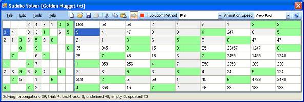
A screen shot of the Sudoku Solver in action is shown above.
The programme displays a single
form with a menu and tool bar at the top and a status bar at the bottom. The centre of the form displays two grids of
9x9 cells. The leftmost one allows you
to enter a puzzle using the keyboard, and displays the final solution. The rightmost one shows the state of the
cells during the calculation in terms of their possible values – if for example
a particular cell could contain the values 2, 5 or 8 then this grid would
display 258 for that cell.
The most important tool bar
button displays a right pointing arrow ![Image 2]() , and this initiates the calculation of the
solution. In order to illustrate the
inner workings of the algorithm it is animated – the cell currently under
consideration is highlighted, and the display updates as new cell values are
calculated. Each cell is colour coded as
follows:
, and this initiates the calculation of the
solution. In order to illustrate the
inner workings of the algorithm it is animated – the cell currently under
consideration is highlighted, and the display updates as new cell values are
calculated. Each cell is colour coded as
follows:
| Initial values
| Pale Green
|
| Calculated values
| Light Cyan
|
| Cells with no possible value
| Pink
|
The red-square button ![Image 3]() can be
used to stop the solving process. There
is also a combo-box allowing you to select the speed of the animation.
can be
used to stop the solving process. There
is also a combo-box allowing you to select the speed of the animation.
I find the animation effect
strangely hypnotic. Or perhaps the
medication is wearing off; <i
>Nurse!
There is also a combo-box which
allows you to choose the solution method – but more on that later.
Saving and Loading to
Text files
Puzzles can be saved to a text file and re-loaded. A selection of prepared puzzles has been
included in the download. The files are
in a simple text format, best illustrated by an example:
; Sudoku file written 09/02/2006 20:00:59.
1.....7..
2........
...3.....
78..6....
...4...3.
.........
.341...5.
.5..786..
.........
Lines beginning with a semi-colon
are treated as comments. The rest of the
file consists of 9 lines of 9 characters, one character for each cell. Undefined cells contain a dot character.
The Solver Algorithm
The solver uses two methods to
find a solution – trial and error and constraint propagation. The ‘Solution Method’ combo-box allows you to
configure what combination of methods to use.
Trial and Error, or Brute Force and Ignorance
The trial and error method is
very straightforward – we generate a possible solution, and test it to see if
it is correct. If it is we are finished,
otherwise we generate another one and repeat.
So this method is often referred to as ‘Generate and Test’.
For the Sudoku solver we use a recursive
version of this, along the following lines:
Function TrialAndError
	Test whether the current grid is valid
	If it is not, return an error code.
	Pick an unallocated cell
	For each possible value for that cell.
		Remember the current state of the grid
		Set the value of the cell to the next possible value
		Call TrialAndError recursively
		If on return we have successfully found a solution
                    Return ‘success’.
		Otherwise reset the grid to its previous state
	Repeat for next possible value
This process is guaranteed to
find a solution eventually, but could take a considerable time. In the very worst case we would have to test
every unallocated cell with the values 1 to 9 recursively. So with 64 un-allocated cells we could try 9
to the power 64 possibilities, which is a huge number – about 1063. The universe would end before we finish. Luckily in practice it’s never as bad as
this, but even so this brute-force approach can take considerable time (see section
on timings below).
Constraint Propagation - Trimming the Possibilities
The problem with the
trial-and-error method discussed above is that we end up having to test many
configurations of the grid which are invalid.
Constraint propagation is a technique for reducing the possible values
we have to test, so speeding up the search for a solution. It is a term from the field of Constraint
Programming – an advanced technique for solving large, complex problems. In Constraint Programming a <i
>constraint is simply a relationship
between two or more variables that
limit their values in some way. Each <i
>variable belongs to a <i
>domain – its set of possible
values. So in the case of Sudoku the
variables are the cells of the grid, the domain of the
variables is the integers from 1 to 9, and the constraints are the rules
that the cells of a row, column or sub-square must be unique.
To propagate the constraint means
to use it to reduce the possible values of a variable. So for example, here is the grid of
possibilities at the start of solving the puzzle shown above:
| 1
| 123456789
| 123456789
| 123456789
| 123456789
| 123456789
| 7
| 123456789
| 123456789
|
| 2
| 123456789
| 123456789
| 123456789
| 123456789
| 123456789
| 123456789
| 123456789
| 123456789
|
| 123456789
| 123456789
| 123456789
| 3
| 123456789
| 123456789
| 123456789
| 123456789
| 123456789
|
| 7
| 8
| 123456789
| 123456789
| 6
| 123456789
| 123456789
| 123456789
| 123456789
|
| 123456789
| 123456789
| 123456789
| 4
| 123456789
| 123456789
| 123456789
| 3
| 123456789
|
| 123456789
| 123456789
| 123456789
| 123456789
| 123456789
| 123456789
| 123456789
| 123456789
| 123456789
|
| 123456789
| 3
| 4
| 1
| 123456789
| 123456789
| 123456789
| 5
| 123456789
|
| 123456789
| 5
| 123456789
| 123456789
| 7
| 8
| 6
| 123456789
| 123456789
|
| 123456789
| 123456789
| 123456789
| 123456789
| 123456789
| 123456789
| 123456789
| 123456789
| 123456789
|
Consider the first cell at (0,0) with the value 1.
The uniqueness rules mean that no other cell in the same row, column or
sub-square can have the same value, so we can remove the value 1 from the
possibilities for those squares. Here’s
the appearance of the grid after we have done this:
| 1
| 23456789
| 23456789
| 23456789
| 23456789
| 23456789
| 7
| 23456789
| 23456789
|
| 2
| 23456789
| 23456789
| 123456789
| 123456789
| 123456789
| 123456789
| 123456789
| 123456789
|
| 23456789
| 23456789
| 23456789
| 3
| 123456789
| 123456789
| 123456789
| 123456789
| 123456789
|
| 7
| 8
| 123456789
| 123456789
| 6
| 123456789
| 123456789
| 123456789
| 123456789
|
| 23456789
| 123456789
| 123456789
| 4
| 123456789
| 123456789
| 123456789
| 3
| 123456789
|
| 23456789
| 123456789
| 123456789
| 123456789
| 123456789
| 123456789
| 123456789
| 123456789
| 123456789
|
| 23456789
| 3
| 4
| 1
| 123456789
| 123456789
| 123456789
| 5
| 123456789
|
| 23456789
| 5
| 123456789
| 123456789
| 7
| 8
| 6
| 123456789
| 123456789
|
| 23456789
| 123456789
| 123456789
| 123456789
| 123456789
| 123456789
| 123456789
| 123456789
| 123456789
|
We can repeat this process for
each cell in the grid with a defined (single) value. Eventually we remove so many possible values
that some new cells also contain a single value. This applies to cell (7,0)
in this grid – it has reduced to the value 9:
| 1
| 469
| 35689
| 25689
| 24589
| 24569
| 7
| 24689
| 2345689
|
| 2
| 4679
| 356789
| 56789
| 14589
| 145679
| 134589
| 14689
| 1345689
|
| 45689
| 4679
| 56789
| 3
| 124589
| 1245679
| 124589
| 124689
| 1245689
|
| 7
| 8
| 12359
| 259
| 6
| 12359
| 12459
| 1249
| 12459
|
| 569
| 1269
| 12569
| 4
| 12589
| 12579
| 12589
| 3
| 1256789
|
| 34569
| 12469
| 123569
| 25789
| 123589
| 123579
| 124589
| 1246789
| 12456789
|
| 689
| 3
| 4
| 1
| 29
| 269
| 289
| 5
| 2789
|
| 9
| 5
| 129
| 29
| 7
| 8
| 6
| 1249
| 12349
|
| 689
| 12679
| 126789
| 2569
| 23459
| 234569
| 123489
| 124789
| 1234789
|
We can then continue the process and propagate the values of
those cells too.
| 1
| 469
| 35689
| 25689
| 24589
| 24569
| 7
| 24689
| 2345689
|
| 2
| 4679
| 356789
| 56789
| 14589
| 145679
| 134589
| 14689
| 1345689
|
| 4568
| 4679
| 56789
| 3
| 124589
| 1245679
| 124589
| 124689
| 1245689
|
| 7
| 8
| 12359
| 259
| 6
| 12359
| 12459
| 1249
| 12459
|
| 56
| 1269
| 12569
| 4
| 12589
| 12579
| 12589
| 3
| 1256789
|
| 3456
| 12469
| 123569
| 25789
| 123589
| 123579
| 124589
| 1246789
| 12456789
|
| 68
| 3
| 4
| 1
| 29
| 269
| 289
| 5
| 2789
|
| 9
| 5
| 12
| 2
| 7
| 8
| 6
| 124
| 1234
|
| 68
| 1267
| 12678
| 2569
| 23459
| 234569
| 123489
| 124789
| 1234789
|
Here is the example on completion
of this propagation process:
| 1
| 69
| 35689
| 68
| 2458
| 2459
| 7
| 2689
| 245689
|
| 2
| 679
| 35689
| 678
| 1458
| 14579
| 134589
| 689
| 145689
|
| 4
| 679
| 5689
| 3
| 1258
| 12579
| 1589
| 2689
| 125689
|
| 7
| 8
| 2
| 9
| 6
| 35
| 45
| 1
| 45
|
| 5
| 169
| 69
| 4
| 128
| 127
| 89
| 3
| 2689
|
| 3
| 1469
| 69
| 78
| 1258
| 1257
| 4589
| 26789
| 245689
|
| 8
| 3
| 4
| 1
| 9
| 6
| 2
| 5
| 7
|
| 9
| 5
| 1
| 2
| 7
| 8
| 6
| 4
| 3
|
| 6
| 2
| 7
| 5
| 34
| 34
| 189
| 89
| 189
|
There is an additional way of applying the uniqueness constraints
which is called the ‘unique value’ rule.
Consider the first row of the possible values:
| 1
| 69
| 35689
| 68
| 2458
| 2459
| 7
| 2689
| 245689
|
The third cell along is the only one
to contain the value 3. This means that
the cell must be the only cell that can
have the value 3 (otherwise it would appear in the possibilities of some other
cell). So if we detect this situation,
either for a row, column or sub-square, we can then force the cell to have that
value, and again continue the propagation.
By applying this method we can further reduce the example grid to the
following possibilities:
| 1
| 9
| 3
| 6
| 458
| 25
| 7
| 28
| 458
|
| 2
| 6
| 58
| 7
| 1458
| 159
| 3
| 89
| 14589
|
| 4
| 7
| 58
| 3
| 158
| 1259
| 1589
| 2689
| 15689
|
| 7
| 8
| 2
| 9
| 6
| 3
| 45
| 1
| 45
|
| 5
| 1
| 69
| 4
| 2
| 7
| 89
| 3
| 689
|
| 3
| 4
| 69
| 8
| 15
| 15
| 59
| 7
| 2
|
| 8
| 3
| 4
| 1
| 9
| 6
| 2
| 5
| 7
|
| 9
| 5
| 1
| 2
| 7
| 8
| 6
| 4
| 3
|
| 6
| 2
| 7
| 5
| 3
| 4
| 189
| 89
| 189
|
It is possible to solve some Sudokus purely by this straightforward constraint
propagation. The samples in the download
marked ‘easiest’ can be solved this way.
Even if we don’t reach a solution
by constraint propagation, the key thing is that we have significantly reduced the
possible values of the cells. Some of
the cells have just two possible values, so if we now chose those cells as the
starting point for the trail and error method we only have to generate and test
two possibilities.
Complete Algorithm
Combining the constraint propagation into the trial and
error method yields an algorithm like this:
Function TrialAndError
	Test whether the current grid is valid
	If it is not, return an error code.
	Propagate Constraints
	Pick an unallocated cell with the fewest possible values
	For each possible value for that cell.
		Remember the current state of the grid
		Set the value of the cell to the next possible value
		Call TrialAndError recursively
		If on return we have successfully found a solution
                    Return ‘success’.
		Otherwise reset the grid to its previous state
	Repeat for next possible value
The Code
The code defines two main
classes:
SudokuSolver This defines the state of
the puzzle grid, and the methods for solving it.
SudokuSolverMainForm This displays the state of the grid, and
defines the menu items and toolbar buttons for driving the application.
In other words the code is
divided into a classic model/view dichotomy.
Synchronisation between the view and the model is achieved using
events. The <i
>SudokuSolver class defines two
events:
<i
>Focused This
event is raised when the solver choses a cell for propagation or
trial-and-error.
<i
>Updated This
event is raised when the solver has finished updating the values of cells
following a propagation or trail-and-error iteration.
The main form subscribes to these two events and updates the
appearance of the two display grids when they occur.
To represent the state of each cell of the grid the code
also defines the SudokuCell class. It stores the possible values of the cell
using SetOfInts16, a structure from the ‘sets’ library described in my previous
article. This is essentially a
bit-array, using one bit to represent the presence of each integer from the
range 0-15.
The key method of the SudokuSolver class is not
surprisingly called Solve:
public bool Solve()
{
Start();
if (!Check())
return false;
return SolveInternal();
}
This does some housekeeping, then
calls an internal method that does the real work:
private bool SolveInternal()
{
    UpdateCounts();
    if (!NoPropagation)
        Propagate();
    if (undefinedCells > 0 && emptyCells == 0 && !stopFlag)
        TrialAndError();
    return (undefinedCells == 0);
}
The <i
>UpdateCounts method calculates
how many cells are still undefined or are empty (have no solution). These counts are used to terminate the solver
when either a solution is found or there are no possible solutions. As you can see from the above, the solver
returns true if there are no undefined cells left – i.e. we have found a
solution.
The Propagate
method keeps propagating the value of known cells until we either
solve the puzzle, detect a cell with no possible values, or cannot find
any more cells to propagate.
Finally the TrailAndError method
implements the ‘generate and test’ algorithm to search for a solution:
private bool TrialAndError()
{
if (NoTrialAndError)
return false;
int row=0;
int col=0;
SudokuCell[,] saved_cells = new SudokuCell[9, 9];
SaveCells(saved_cells);
if (FindBestTrialCandidate(ref row, ref col))
{
SudokuCell x = cells[row, col];
foreach (int i in x)
{
trialCount++;
OnFocus(row, col);
cells[row, col].Value = i;
OnUpdate();
bool bValid = true;
if (NoPropagation)
bValid = Check(row, col, i);
if (bValid)
{
if (SolveInternal())
return true;
RestoreCells(saved_cells);
}
backtrackCount++;
if (stopFlag)
return false;
}
}
return false;
}
The
method FindBestTrailCandidate
searches the grid
for the best candidate for trial-and-error.
We try to find the cell with the fewest possible values. If we find a cell with just two possible
values we can use that one without
further search.
For more information look at the supplied source – I hope it
is sufficiently self-explanatory.
Timing Comparison
In order to back up my assertion
as to the superiority of constraint propagation I gathered some timing statistics
for various sample puzzles:
| Sudoku Puzzle
| Trail and error only
| Trail and error plus propagation
| Speed Increase factor
|
| Sudoku 00 empty
| 0.137 secs
| 0.333 secs
| 0.374
|
| Sudoku 01 easiest
| 0.0262 secs
| 0.0092 secs
| 2.856
|
| Sudoku 03 diabolical
| 0.936
| 0.0554
| 16.887
|
| Sudoku 05 easy
| 10 hr 21 m 35 s
| 0.017 secs
| 2486769.9
|
| Sudoku 98 Easter Monster
| 66.675 secs
| 0.848 secs
| 76.993
|
| Sudoku 99 Golden Nugget
| 65.3 secs
| 2.051044
| 31.837
|
Puzzle 00 is the empty grid. For this puzzle the constraint propagation
method is slower than the trial and
error method, as there are no initial constraints. However, for all the
true puzzles the constrain propagation method beats the pure trial and error
method by a significant factor. The
extreme example of this is the puzzle introduced in the first section – number
5. To solve this by trial and error
takes over 10 hours on my laptop! You
can see why this might be if you look at the solution. The first unallocated cell is the second
square on the top row, and in the solution this has the value 9. So in order to reach this the trial and error
method must run through every possible combination until it reaches a 9 in this
cell. This takes over <b
style='mso-bidi-font-weight:normal'>one
billion iterations.
Real World Applications of Constraint Programming
I’ve tried to show how Constraint
Programming can be applied to a familiar example, but there are many real-world
applications in which it can be used. For
example there are working systems in the following areas:
- Picture
recognition.
- Creating
schedules for airlines, bus and train companies.
- Placing
transmitters for Cellular radio.
- DNA
sequencing.
- Electronic
circuit design.
You can find lots more information on the web – there are
some links at the end of the article.
Summary
I know this is at least the 24th
Sudoku article on CodeProject. I hope this one is sufficiently different
that you do not feel you have wasted your time reading it. Thank you.
Further <st1:city w:st="on"><st1:place w:st="on">Reading
Postscript
Sisyphus was the legendary Greek
king condemned by the gods to push a boulder uphill for all eternity. Whenever he reached to hilltop the bolder
rolled back down to the bottom. Hence a
Sisyphean task is both arduous and futile.
License
This article, along with any
associated source code and files, is licensed under <a
href="http: www.codeproject.com="" info="" cpol10.aspx"="">The
Code Project Open License (CPOL)
History
- Initial
version 15 February 2009
I have been working in IT since 1975, in various roles from junior programmer to system architect, and with many different languages and platforms. I have written shedloads of code.
I now live in Bedfordshire, England. As well as working full time I am the primary carer for my wife who has MS. I am learning to play the piano. I have three grown up children and a cat.


 General
  News
News  Suggestion
  Question
  Bug
Bug  Answer
  Joke
Joke  Praise
  Rant
Rant  Admin
Admin 


