
Machine Learning in Parallel with Support Vector Machines, Generalized Linear Models, and Adaptive Boosting
ML methods using bootstrap samples and parallel processing to model very large volumes of data in short periods of time
Introduction
This article describes methods for machine learning using bootstrap samples and parallel processing to model very large volumes of data in short periods of time. The R programming language includes many packages for machine learning different types of data. Three of these packages include Support Vector Machines (SVM) [1], Generalized Linear Models (GLM) [2], and Adaptive Boosting (AdaBoost) [3]. While all three packages can be highly accurate for various types of classification problems, each package performs very differently when modeling (i.e., learning) different volumes of input data. In particular, model fitting for Generalized Linear Models execute in much shorter periods of time than either Support Vector Machines or Adaptive Boosting. In instances where very large datasets must be fitted, learning times for both ADA and SVM appear to grow exponentially rather than in a linear fashion. However, when using a combination of parallel processing and bootstrap sampling, all three machine learning methods can be tuned for optimal performance on both the Linux and Windows platforms.
About the Models
After looking at the general algorithms supporting each of these models, it quickly becomes obvious why the Generalized Linear Models perform so much faster when training on larger volumes of data. While GLM performs a more simplistic linear regression using a set of observed values to predict its response variable, the algorithms for both SVM and ADA deploy much more sophisticated techniques. Support Vector Machines are a form of non-probabilistic binary linear classifiers [4] which fit a “maximum-margin hyperplane in a transformed feature space” [4]. The creators of SVM, Cortes &Vapnik (1995) [1,5], describe this process as “class separation” which means “looking for the optimal separating hyper-plane between two classes by maximizing the margin between the classes’ closest points”. [1] When using the popular Radial Basis Function kernel, the corresponding feature space is “a Hilbert space of infinite dimensions”. [4] Adaptive Boosting works by taking misclassified examples from previous learning iterations and assigning them higher weights in subsequent iterations. [6] This process is called “iterative re-weighting”, and it is crucial to the success of Adaptive Boosting. [6]

Bootstrap Sampling
The process of bootstrap sampling allows estimation of a data population’s variance by “measuring those properties when sampling from an approximating distribution”. [10] In simplistic terms, this means that just because you have collected or randomly sampled some data, your particular data’s unique characteristics do not necessarily represent all of the unique characteristics that could be observed when examining all possible instances of the type of data which you have collected. For example, let's imagine that I have borrowed five different randomly chosen Mercedes Benz model C250 vehicles from the Mercedes dealership for observation (lucky me!). It is obvious that I would be missing many colors and options from the entire C250 lineup. Furthermore, if I randomly sampled 20 vehicles from the same dealership’s lot at different times of the year, I may draw very different conclusions about the most common colors, options, and vehicle models offered by that particular dealer. Bootstrapping is a technique which can assist with smoothing out some of these unintended variances in your data bringing greater stability to any conclusions drawn.
In machine learning, Bootstrapping is a great technique to avoid over-fitting your model to a particular set of training data. A modeling process which is trained on or utilizes the results from multiple bootstrap samples will typically “generalize” better making more accurate predictions when classifying against many different sets of input data. When referring to Figure 1, imagine that the lines drawn for any given machine learning method displayed are very specific to the particular set of data provided during training. Now, imagine that the actual line for all possible instances of this type of data looks similar but varies at different points on the curve. This means that the model will be over-fitted and not generalize very well when making classifications. Bootstrapping can be thought of in a manner similar to the Adaptive Boosting iteration images in that the different bootstrap samples can be used as yet another method to appropriately adjust the classification line for more accurate results.
One of the most powerful features of Bootstrapping during machine learning is that some given populations of training data are simply too large for more complex machine learning methods such as SVM and AdaBoost. In these situations, multiple bootstrap samples can be taken to build a highly accurate and responsive modeling process using much smaller randomly sampled subsets of the input data. Furthermore, the optional prediction probabilities returned by most machine learning packages in R (including GLM, SVM, and AdaBoost) can be used to rank individual bootstrap predictions so that multiple model results can be combined for a prediction consensus between any number of bootstrap samples and even different machine learning packages. Creating n bootstrap samples for the purposes of machine learning is a very simple process which typically comprises taking n equally sized random samples with replacement from the input dataset which are then subsequently used for training purposes during machine learning.

(Click image to cut and paste code)
Parallel Processing in R
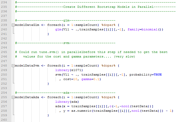
The R Programming Language offers multiple solutions for symmetric multiprocessing (SMP). SMP is a form of parallel processing using multiple processors which all connect to a single shared main memory. Parallel processing for both Linux and Windows platforms can easily be supported in R with very minor program modifications. The doMC [11] and doSNOW [12] packages in R offer a very simple loop construct foreach which executes in parallel when the %dopar% directive is used. Furthermore, the foreach construct is near identical in both packages requiring only minor setup changes when porting code between Linux and Windows. Although some machine learning algorithms such as SVM are not easily implemented in parallel, multiple SVM training processes against bootstrap samples can easily be executed in parallel drastically reducing overall training time requirements.

(Click image to cut and paste code)

(Click image to cut and paste code)
It is important to mention that “parallel” is not always better. In many cases, the overhead and time required for breaking a task into individual, independent units of parallel work and creating threads or forking processes is much greater than just simply executing the task on a single processor. Furthermore, parallel processing can quickly become very complex and error prone introducing deadlocks and race conditions into code that previously executed bug free in a single processor environment. However, some tasks show huge parallel performance gains when implemented correctly. Figure 6 below documents the Generalized Linear Model under-performing substantially with processing time increasing by over 100% when executed in parallel. However, both SVM and AdaBoost post huge performance gains when running in parallel with SVM training almost 4 times faster.

A Practical Example
The University of California at Irvine maintains a large collection of machine learning databases which are useful for testing purposes. The following practical example demonstrates using the UCI Magic Gamma Telescope dataset with the GLM, SVM, and AdaBoost machine learning packages in R. Multiple bootstrap samples are created, and then each bootstrap is trained and tested in parallel using each machine learning package. Test results demonstrate that comparable accuracy results can be achieved using as few as 8 random bootstrap samples of only 20% (with replacement). In addition, utilizing the bootstrap samples allows model training to occur in parallel and produces large performance gains in most cases. It is important to mention, as we will soon find out, that bootstrapping does not always produce optimal results for both speed and accuracy. When possible, bench-marking should be performed to determine the best implementation method.

(Click image to cut and paste code)
(Click image to cut and paste code)

(Click image to cut and paste code)
Ranking Predictions for Multiple Bootstrap Models
When using bootstrap samples, making blended class predictions can be accomplished by simply counting each bootstrap model’s predicted class for a given input and determining the final blended class assignment using a voting scheme between bootstrap models. For example, if 4 models predict True and 1 model predicts False, the blended prediction is True by a vote of 4 to 1. Furthermore, blended confidence for a particular class can be determined by using a ranking procedure where all bootstrap predictions are ranked based on the probability of a given class. Once ranks have been assigned, they can easily be added together to compute a final ranking for each prediction’s likelihood of belonging to a specific class. This is useful when it is important to understand the confidence for each membership prediction compared to all other predictions.

(Click image to cut and paste code)

(Click image to cut and paste code)
Results
The final results demonstrate that comparable accuracy can be achieved using as few as 8 random bootstrap samples of only 20%. Furthermore, both the SVM and ADA models boast very large performance gains during training by taking advantage of parallel processing against smaller volumes of input data. It is important to mention that while all of the elapsed execution times are very close to (or less than) one minute using the Magic Gamma Dataset, the exponential growth of training performance times for both SVM and ADA make these performance gains even more substantial when fitting larger volumes of data. Likewise, it is important to recognize that the parallel processing performance break-even point for the GLM model is much higher. No parallel processing training benefits are gained in the case of GLM when using this dataset. One small drawback related to bootstrapping is that prediction processing inputs increase by a factor of 8 in this example, since 8 bootstraps were used. Each classification must be made using each of the 8 bootstrap models. Elapsed time differences for predictions are minimized by using parallel processing. However, classification times for the bootstrapping process are slightly slower. Fortunately, prediction processing times do not appear to grow exponentially based upon input data volumes like the ADA and SVM training times do. In the case of ADA and SVM, attempted training against as few as 250,000 records may cause the training process to never complete. At this point, bootstrapping is not only optimal, but it is the only option described in the article that will still work.

Further gains in accuracy can also be achieved when looking at a particular class of predictions. When predictions are ranked and sorted by the probability of a given class, higher accuracy thresholds can be set by only selecting higher ranking subsets of a particular class. For example, selecting only the top 175 ranking predictions for the class “g” yields a prediction accuracy of 100% for both SVM and ADA. Selecting the top 1500 highest ranking predictions for the class “g” increases accuracy by an average of 9.3% across all models.

Stacking Bootstrap Results
Using the blended bootstrap model rankings above, additional increases in classification accuracy and class prediction volumes can still be achieved by stacking the results from each machine learning package. Since GLM, SVM, and ADA each use different techniques for classification, top rankings will not be identical across all three prediction populations. For instance, SVM achieves the highest accuracy score of all three machine learning packages at 93.4% when looking at the top 2,000 highest ranking predictions. Furthermore, the ADA and GLM packages score above 93.4% accuracy when looking at the top 1,500 and 100 predictions respectively.


(Click image to cut and paste code)
Resources
- All programming code used for this article can be accessed at http://jakemdrew.com/blog/watson.htm
References
- David Meyer, Support Vector Machines, http://cran.at.r-project.org/web/packages/e1071/vignettes/svmdoc.pdf, accessed on 03/06/2014.
- German Rodriguez, Generalized Linear Models, http://data.princeton.edu/R/glms.html, accessed on 03/06/2014.
- Mark Culp, Kjell Johnson, and George Michailidis, Package ‘ada’, http://cran.fhcrc.org/web/packages/ada/ada.pdf, accessed on 03/06/2014.
- Wikipedia, Support Vector Machines, http://en.wikipedia.org/wiki/Support_vector_machine, accessed on 03/07/2014.
- Cortes, C. & Vapnik, V. (1995). Support-vector network. Machine Learning, 20, 1-25.
- Meir, R., & Rätsch, G. (2003). An introduction to boosting and leveraging. In Advanced lectures on machine learning (pp. 118-183). Springer Berlin Heidelberg.
- perClass, Support Vector Classifier, http://perclass.com/doc/guide/classifiers/svm.html, accessed on 03/07/2014.
- Wikipedia, Generalized Linear Models, http://en.wikipedia.org/wiki/Generalized_linear_model, accessed on 03/07/2014.
- Statistical Machine Learning and Visualization At the Georgia Institute of Technology, Linear Regression and Least Squares Estimation, http://smlv.cc.gatech.edu/2010/10/06/linear-regression-and-least-squares-estimation/, accessed on 03/07/2014.
- Wikipedia, Bootstrapping, http://en.wikipedia.org/wiki/Bootstrapping_(statistics), 03/07/2014.
- Steve Weston, Getting Started with doMC and foreach, http://cran.r-project.org/web/packages/doMC/vignettes/gettingstartedMC.pdf, accessed on 03/07/2014.
- Steve Weston, Package ‘doSNOW’, http://cran.at.r-project.org/web/packages/doSNOW/doSNOW.pdf, accessed on 03/07/2014.
