
Slaving Over a Hot Laptop,PID control loops and Sous Vide cooking
PID thermal control loop simulation

Introduction
I can do most things with my laptop, why can’t I make it cook? I’ve attached sensors, motors, NMR, cameras, etc. why not a heater and a thermometer?
Sous Vide, or immersion cooking produces great tasting food. It is also an interesting representative problem of closed loop temperature control. With numerous people trying to provide an open source or DIY solution for Sous Vide cooking, I figured I’d add to that body of work in my own way. I’d write a software simulation of an immersion cooker to help people develop better hardware. I don’t know what the time constants in the simulation might be, but you can set them, and learn PID control. I also might hook up a relay, a heater, and a thermo couple and actually do this, but mostly I figured I’d help others study basic PID control.
Background
PID control loops (Proportional, Integral, Derivative) are a basic form of closed loop control, meaning the error is fed back into the control loop and used to change how control is performed as opposed to open loop.

In a PID loop, an error is calculated, and then three different terms are computed and summed to form a correction. The incoming error term may have known properties based on how the measurement was made or changes to the goal value, so sometimes pre-filtering is performed (FIR/IIR). The integral sometimes isn’t truly just adding up the errors but sometimes decays so it has a limited memory of past errors. The derivative term may be subtracting two noisy errors that are similar producing a large value that is mostly noise so sometimes the derivative value is filtered (FIR /IIR, outlier rejection, boxcar, etc.).
Finally each of these terms may have a dead band, and the sum may too. A dead band means don’t adjust unless over +X threshold amount, or under –Y threshold amount. Further the control applied may also be filtered to remove control changes that would cause a harmonic pattern, such as oscillation.
So with this in mind, a generic PID may have a large set of features (pre/post filters), dead bands, and pre /post conditioning filters, and a variety of integration like effects.
PID Tuning
In general, a PID filter can be thought of as a corrective loop, where you move closer to the goal proportional to the error perceived. In many cases a proportional gain is what’s needed. For example for servo motion where there is a large motor and a tiny weight, driving to position requires only a P term. If there is consistent pressure (weight) or loss (heat loss) proportional control may not be enough. The integral term adds up tiny errors, and corrects better than proportional when the error is small. The integral term may accelerate too much resulting in over correction and even oscillation, so the derivative term is then used like a break.
There are several tuning techniques, the author prefers starting with Ziegler-Nichols. I set the proportional gain till it over controls resulting in oscillations I can measure. When the system is mostly linear, the oscillations will have fixed period. This proportional gain is the “ultimate” gain or Ku, and the period is Pu. From there:
P only: P = 0.5*Ku
PI only: P = 0.45*Ku, I = 0.54*Ku / Pu.
PID: P = 0.6*Ku, I= 1.2*Ku/Pu, D = 0.075*Ku*Pu
In most cases, this is close to good enough. In the case of a Sous Vide, overshoot (going too hot while attaining a temperature) is bad, and consistent undershoot is bad. It can take a known time to reach stability before we put the food in is ok. For this reason, backing off on I and D terms, and using a decaying integral are likely good ideas.
There are many systems to compute “ideal” coefficients but they don’t arrive at the same answer, go figure. Ideal is based on your particular requirements, and simulation helps a lot. Integrating with the real system then tells you how much more work to do, it usually isn’t a check the box test unless you’re lucky or the control system was simulated perfectly, or it is relatively linear and or simple. Most problems I’ve used PID on started simple, then weight was cut, materials changed, etc. and at some point simulation became just a starting point. At some point PID stops working and a lookup table based on measurements for coefficients to interpolate from is required. That is the essence of an autopilot because that kind of algorithm can model non-linear processes that appear linear or quadratic over short numerical regions (perhaps a different article). My point is, PID usually can solve the problem if the problem is reasonable but there are other solutions that sometimes work better.
If your problem seems too hard to solve because small changes in gains cause the system to behave strangely then likely there is a non-linear response to the correction and PID might not be the choice to use.
For Sous Vide cooking, temperature isn’t linear in time (exponential) but it is a smooth effect, and over any short region of change if we treat it as linear, the error term isn’t huge or suddenly change sign. For those reasons PID will work, perhaps not ideally converging with zero overshoot but it works very well and is probably the most common way to handle heating control.
Requirements
The key thing is to bring food up to a target temperature ideal for that food, and hold it there for a period of time. For example to cook an egg so only certain proteins coagulate (perfect poached egg), or to make the perfect steak, or carrots, the food is cooked longer than needed at no more than the set temperature, and as close to the set temperature as possible. Above certain temperatures the heat only breaks down flavor and makes the food tougher for certain foods.
Temperature:
Min, Max. 1000F to 2200F (roughly 500C to 1000C)
Accuracy 0.250F (threshold) 0.10F (goal)
Stability Gaussian 1-sigma of accuracy to time constant of heat transfer.
Overshoot Initial overshoot of water ok if food isn’t present.
Need to know when food started to be at temperature to know how long to cook it.
Physical Control:
Either proportionally or pulse an AC heater. Pulsing with a solid state relay is probably cheapest, but the frequency of the pulses need to be realistic because they affect how well the heating element will accurately respond and the life of the heating element.
Physics

Model Assumptions
- Heater has a metal outside surface.
- Water is circulated rapidly to avoid significant gradients
- Inside of container is metal or water is circulating so container is a uniform effect on the water.
- Container is an insulator.
- Bag is slightly an insulator.
- Air temperature is room temperature, uniform (enough).
- Anything that is relatively uniform or circulates faster than the time constant of transfer to it is equivalent to uniform.
- Relative time constants:
Slow -> Container/Air -> Container/Water -> Medium ->Bag/Food -> Others -> Fast
Math

Math References
http://en.wikipedia.org/wiki/Heat_transfer
http://en.wikipedia.org/wiki/Specific_heat_capacity
http://en.wikipedia.org/wiki/Fourier%27s_Law
http://en.wikipedia.org/wiki/PID_controller
Mathematics of Physics and Modern Engineering, McGraw hill publishing, 1966, by I.S. Sokolnikoff & R.M. Redheffer, p. 432.
Indroduction to Applied Mathematics, Wellesly-Cambridge Press, 1986, by Gilbert Strang, p. 461, 536.
Simulation
The model can be describes as a set of heat transfers. Yes, the specific heat and energy could be modeled with a more classical thermodynamic model, but in the end the math reduces more or less to time constants and transfer from one singular thermal body to another.
The heat escape path is: Water-> Container -> Air && Water->Air.
The add path is: Heater-> Water
The measurement path is: Water-> Sensor
We can turn what could be a wacky looking differential equation into a set of difference equations .
By making the simulation time arbitrarily small, the error is arbitrarily small, and computers are good at rapid repeated calculations. For this reason, FEA modeling or differential equations are just not needed (although a lot of fun, but not in this article). In short we can simulate multiple simultaneous heat transfers as heat adding or being lost across a given boundary, rewriting as a difference:

Because the volume of water is varying, assuming a pot or rice cooker we can adjust the time constant based on the surface area to volume ratio and simulate those affects. We can also run the adjustment times at a different rate to the simulation time delta, and set weather control is proportional or pulsed and compare the results.
Water volume effect:

Code
private void simulateTime(double dt, double percentHeat, ref double water, ref double container, <br /> ref double sensor, ref double food, Parameters p, PID pid, bool usePID)
{
// Limit to the max / min.
percentHeat = percentHeat < 0 ? 0 : percentHeat > 100 ? 100 : percentHeat;
// If binary, heater is on/off in which case threshold.
if (p.Binary) { percentHeat = percentHeat > 25 ? 100 : 0; }
double heaterAdded = percentHeat * p.HeaterWatts * heaterSpecificHeatFactor;
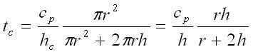
// surface area is constant but thermal mass of the water isn't.
double effectiveWaterContainer = p.TWC * p.WaterRadius * p.WaterDepth /
(p.WaterRadius + 2 * p.WaterDepth);
double effectiveWaterAir = p.TWA * p.WaterDepth;
// Heat added from heater to water.
double heatAddedToWater = (heaterAdded - water) *
(1 – (1/ p.TWH) * System.Math.Exp(-dt / p.TWH));
heatAddedToWater = heatAddedToWater < 0 ? 0 : heatAddedToWater;
// Heat lost to the sensor.
double heatLostToSensor = (water - sensor) * (1-System.Math.Exp(-dt / p.TWS))/p.TWS;
// Heat lost to the food.
double heatToFood = (water - food) * (1 - System.Math.Exp(-dt / p.TWF)) / p.TWF;
// Heat from water to container.
double heatLostWaterContainer = (water - container) *
(1 - System.Math.Exp(-dt / effectiveWaterContainer))/effectiveWaterContainer;
// Heat water to air.
double heatLostWaterAir = (water - p.Air) *
(1 - System.Math.Exp(-dt / effectiveWaterAir))/effectiveWaterAir;
// Heat Container to air.
double heatLostContainerAir = (container - p.Air) *
(1 - System.Math.Exp(-dt / p.TCA))/p.TCA;
// Update.
food = food + heatToFood;
water = water + heatAddedToWater - heatLostWaterContainer –
heatLostWaterAir - heatLostToSensor - heatToFood;
sensor = sensor + heatLostToSensor;
container = container + heatLostWaterContainer - heatLostContainerAir;
}
public class PID
{
double m_p = 0, m_i = 0, m_d = 0, m_g = 0, integral = 0, last = 0;
bool first = true;
public PID(double setPoint, double proportional, double integral, double derivative)
{
m_g = setPoint; m_p = proportional;
m_i = integral; m_d = derivative;
}
public double Update(double sensor, double dt)
{
double error = m_g - sensor;
integral = (0.9 * integral) + error;
double derivative = first ? 0 : (sensor - last) / dt;
last = sensor;
first = false;
return (m_p * error) + (m_i * integral) + (m_d * derivative);
}
}
Results
The following time constants in seconds were guessed at to produce are somewhat realistic simulation:
Water-heater 600
Water-sensor 2
Water-container 1000
Container-air 1000
Water-food 20
Water-air 1000
Sure the time constants are made up. After gathering actual data, make educated guesses. For anything I’ve worked on (missiles, GPS motion, thermal control) it was always an estimate, a guess, the reality is even if you measure the exact value, when you get to production there is enough variation for the exact value not to matter. Simulation tied to real data ensures that if the production values vary, the gains provide for robust control anyways. One of the best ways to do this for real would be to turn the heater on at various fixed values and measure the steady state water and container temperatures, and look up the time constant for the thermocouple used, then make the model look like the curves seen for real, double checking with heat loss vs. heat added. Pure math often won’t do all the work unless your system is simple and well known (density of the plastic container, exact CAD model for shape, calibrated heater wattage, losses in switching on/off, etc.).
It took a proportional gain of over 100 to start to see an initial overshoot, the inherent decay meant there is no real gain that will cause an oscillation. Using Ziegler-Nichols, and looking at the overshoot, the time to decay from an overshoot is in tens of seconds so IF Pu did exist it would be on the order of 5-20 seconds, and our gain ultimate (Ku) can be large (10 – 50). This provides ball park initial values to setup and study (Ku = 30, Pu = 10).
P = 0.6*Ku, I= 1.2*Ku/Pu, D = 0.075*Ku*Pu
P = 18, I = 3.6, D = 22.5
This resulted in the following graph:

The problem is it was 0.2 degrees too cool for the second half of cook time, clearly we need more integral. Doubling the gains brought the system closer (62.69).
Note what happened when I used non-proportional pulsed
control:
Because the food provide a sort of temperature buffer, it takes time to transfer water to food through the bag the food is in, a little water overshoot is desirable if accuracy is improved. For this reason we can play with the numbers and improve performance.
If this was more than an intellectual exercise, the next step would be to randomly generate start water temperatures (which also has the affect of spontaneously adding food a different temperature to the bath after reaching temperature) as well as varying water-food time constant (simulate different volumes of foods, marinades in the food bag). Then show that for a given set of gains there is little overshoot, and very stable performance.
For the most part, most gain choices will be stable enough, but some will get the water to the desired temperature faster than others, and in a commercial kitchen producing product on a time schedule that would mater. For teaching your lap top how to make tuna confit, or perfect harcot verts, a little simulation and some trial and error should be sufficient.
The key result from the simulation suggests using a PID with a simple relay would work very well, and thus a rice cooker plugged into a relay controlled by a PID should (in theory) be sufficient.